Amortization CalculatoR
How to Build Amortization Tables in R
Last year, I bought my first house (huzzah!), and as any respectable useR, I decided I had to create my own amortization tables in R. Taking it a step further, I really wanted to know what the effect of extra payments would be.
Now, I was sure there must be a package already developed to do exactly this, but some quick searching online came up with a lot of web app calculators. I gave up and turned to the learning opportunity that would be writing my own script to accomplish this task.
What the Heck is Amortization, Anyway?
Okay, let’s start out with a big ’ol COA disclaimer right here – I’m no financial advisor, banker, CPA, or even that savvy of an investor. So, I will only provide basic descriptions of financial concepts necessary for us to accomplish the task at hand.
You want to buy a home, but you only have a portion of the total price. So, you go to a bank to get a loan. The bank will give you all the money to buy the home now if you promise to pay that amount – the principal – plus interest in a certain amount of time. You will make monthly payments that are part interest and part principal payments until the full amount of principal is repaid.
If you follow the payment schedule, you will pay a certain amount in interest. This interest rate is variable depending on the amount of outstanding principal, which means if you make extra payments towards principal, there is less interest to be paid.
So, how do you know how much interest you’re paying and how much principal each month? That’s where the amortization table comes in – the table provides the breakdown of interest to principal for each payment. That means our first task is to translate the table calculation into our R script.
Doing the Math
Total Monthly Payments (Principal + Interest)
The following formula calculates the monthly mortgage payment, which includes both the principal and interest:
The code below is the equation translated to R. I’ve also defined the other variables we’ll need with default values.
# Define the variables

term <- 360 # 30 years in months
original_loan_amount <- 150000 # $150,000 loan
annual_rate <- 0.04 # 4% interest rate
monthly_rate <- annual_rate/12 # rate converted to monthly rate

# Formula to calculate monthly
# principal + interest payment

total_PI <- original_loan_amount *
   (monthly_rate * (1 + monthly_rate) ^ term)/
   (((1 + monthly_rate) ^ term) - 1)
In this example, the total monthly payment (i.e. total_PI) is \(\$716.12\), which when multiplied by the term of the loan results in a total payment amount of \(\$257,804.26\) – in other words, over the life of this loan, we’ll be paying \(\$107,804.26\) in interest.
Breakdown of Principal and Interest in Each Payment
The portion of each payment that goes towards the principal – or the original loan amount – is what pays down your loan and builds equity. The portion that goes to interest is the cost you pay for the bank to give you the loan. Basically, the amount of interest you pay each month is determined by multiplying the monthly_rate by the remaining balance of the loan. This number will be less than the total_PI, and whatever the difference is between the two will be the principal portion of the payment.
Since total_PI is fixed and the interest portion of the payment is a function of the remaining loan balance, as you pay down the loan, the portion that goes to interest decreases, which results in a comparable increase in the portion that goes to principal.
Now we’re getting very close to being able to create our amortization table. We know what our total_PI is, so now we just need to write code that will calculate the interest and principal portion of each payment, and then calculate the remaining principal.
The following code will create numberic vectors for each value, with the length of each being set to the term of the loan.
# Initialize the vectors as numeric with a length equal
# to the term of the loan.

interest <- principal <- balance <- date <- vector("numeric", term)

loan_amount <- original_loan_amount
# For loop to calculate values for each payment

for (i in 1:term) {
   intr <- loan_amount * monthly_rate
   prnp <- total_PI - intr
   loan_amount <- loan_amount - prnp

   interest[i] <- intr
   principal[i] <- prnp
   balance[i] <- loan_amount
}

# Throw vectors into a table for easier use

library(tidyverse) # for data manipulation going forward

standard_schedule <- tibble(payment_number = 1:term,
                            interest,
                            principal,
                            balance)

# Print head of standard_schedule

library(knitr) # both libraries for printing tables
library(kableExtra)

standard_schedule %>%

  # Format columns to display as dollars

  modify_at(c("interest", "principal", "balance"), scales::dollar,
            largest_with_cents = 1e+6) %>%

  # Limit to first 10 payments

  head(10) %>%
  kable(booktabs = T) %>%
kable_styling()| payment_number | interest | principal | balance |
|---|---|---|---|
| 1 | $500.00 | $216.12 | $149,783.88 |
| 2 | $499.28 | $216.84 | $149,567.03 |
| 3 | $498.56 | $217.57 | $149,349.47 |
| 4 | $497.83 | $218.29 | $149,131.18 |
| 5 | $497.10 | $219.02 | $148,912.16 |
| 6 | $496.37 | $219.75 | $148,692.41 |
| 7 | $495.64 | $220.48 | $148,471.93 |
| 8 | $494.91 | $221.22 | $148,250.71 |
| 9 | $494.17 | $221.95 | $148,028.76 |
| 10 | $493.43 | $222.69 | $147,806.06 |
With our payments now calculated for the full term of the loan, we can visualize the interest and principal portions in a line graph.
# Pivot longer makes it easier to visualize,
# but isn't totally necessary

standard_schedule %>%
  pivot_longer(cols = c("interest", "principal"),
               names_to = "Payment Portion",
               values_to = "amount") %>%
  ggplot(aes(payment_number, amount, color = `Payment Portion`)) +
  geom_line() +

  # '#85bb65' is the color of $$$

  scale_color_manual(values = c("red", "#85bb65")) +

  # Change the theme for better appearance

  theme_minimal() +
  scale_y_continuous(labels = scales::dollar) +
  labs(title = "Payment Portions of Monthly Mortgage")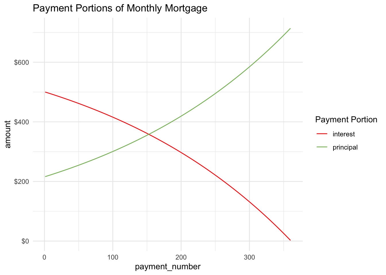
Judging from this visual, we can estimate that the portion of each payment going to principal will exceed the portion going to interest at about the 150th payment. To be exact, we can filter the amortization table to find where principal exceeds interest for the first time.
# Filter for interest less than principal

standard_schedule %>%
  filter(interest < principal) %>%

  # Include only the first observation

  head(1) %>%

  #  Prettify for table

  modify_at(c("interest", "principal", "balance"), scales::dollar,
            largest_with_cents = 1e+6) %>%
  kable(booktabs = T) %>%
kable_styling()| payment_number | interest | principal | balance |
|---|---|---|---|
| 153 | $357.72 | $358.41 | $106,956.13 |
So payment number 153 is the first payment where the portion going to principal is greater than the portion going to interest.
Adding Dates
Now, a natural follow-up question is when will the 153rd payment take place? This is actually an easy question to answer – all we need to do is add a date vector to our table. We will create a variable with the date of the first monthly payment, and then the vector will be a sequence of dates by month for the term of the loan. The following code accomplishes this task.
library(lubridate)

# Set first payment date

first_payment <- "2020-01-01"


# Add vector as variable to standard schedule

standard_schedule <- standard_schedule %>%
  mutate(date = seq(from = ymd(first_payment), by = "month",
            length.out = term)) %>%
  select(date, everything())

standard_schedule %>%
  modify_at(c("interest", "principal", "balance"), scales::dollar,
          largest_with_cents = 1e+6) %>%
  head(10) %>%
  kable(booktabs = T) %>%
kable_styling()| date | payment_number | interest | principal | balance |
|---|---|---|---|---|
| 2020-01-01 | 1 | $500.00 | $216.12 | $149,783.88 |
| 2020-02-01 | 2 | $499.28 | $216.84 | $149,567.03 |
| 2020-03-01 | 3 | $498.56 | $217.57 | $149,349.47 |
| 2020-04-01 | 4 | $497.83 | $218.29 | $149,131.18 |
| 2020-05-01 | 5 | $497.10 | $219.02 | $148,912.16 |
| 2020-06-01 | 6 | $496.37 | $219.75 | $148,692.41 |
| 2020-07-01 | 7 | $495.64 | $220.48 | $148,471.93 |
| 2020-08-01 | 8 | $494.91 | $221.22 | $148,250.71 |
| 2020-09-01 | 9 | $494.17 | $221.95 | $148,028.76 |
| 2020-10-01 | 10 | $493.43 | $222.69 | $147,806.06 |
Now when we look at the 153rd payment, we see the date is September 01, 2032.
standard_schedule %>%
  filter(interest < principal) %>%
  head(1) %>%
  modify_at(c("interest", "principal", "balance"), scales::dollar,
            largest_with_cents = 1e+6) %>%
  kable(booktabs = T) %>%
kable_styling()| date | payment_number | interest | principal | balance |
|---|---|---|---|---|
| 2032-09-01 | 153 | $357.72 | $358.41 | $106,956.13 |
Creating an Adjusted Schedule
Next, we will create an adjusted schedule that accounts for both extra monthly and one-time payments towards principal. With these extra payments, the principal will be paid off before the full term of the loan, and you will therefore pay less interest.
To accomplish this, we will create new variables in our schedule for both extra monthly payments and extra one-time payments. Additionally, we will want to save our adjusted schedule as a different object than standard_schedule so we can compare it to the standard schedule.
# Create new variables for updated schedule

loan_amount1 <- original_loan_amount

interest1 <- principal1 <- extra <- xtra <- balance1 <- bonus <- NULL

# Set the extra monthly payment amount

for (i in 1:term) {

  # Stop the for loop when blance is paid off
  # Otherwise, loop will keep making monthly payments
  # Also must be sure to round values to 0.00

  if(loan_amount1 > 0.00) {
    intr1 <- (loan_amount1 * monthly_rate) %>%

      # Round to 0.00 for payments

      round(2)

    # Last payment won't be in full

    prnp1 <- ifelse(loan_amount1 < (total_PI - intr1),
                    loan_amount1,
                    total_PI - intr1) %>% round(2)

    # Last payment won't need extra payment

    xtra <- ifelse(loan_amount1 < (total_PI - intr1), 0, 100)

    loan_amount1 <- (loan_amount1 - prnp1 - xtra) %>%
      round(2)

    extra[i] <- xtra
    interest1[i] <- intr1
    principal1[i] <- prnp1
    balance1[i] <- loan_amount1
  }
}

# Set new term length

new_term <- length(balance1)

# Combine in single table

updated_schedule <- tibble(date = seq(from = ymd(first_payment), by = "month",
                                      length.out = new_term),
                          payment_number = 1:new_term,
                          interest = interest1,
                          principal = principal1,
                          extra,
                          balance = balance1)
The code above creates the updated_schedule table for us. We can inspect the first ten payments just like we did with the standard_schedule, with the addition of our extra monthly payment.
updated_schedule %>%
  modify_at(c("interest", "principal", "extra", "balance"), scales::dollar,
          largest_with_cents = 1e+6) %>%
  head(10) %>%
  kable(booktabs = T) %>%
kable_styling()| date | payment_number | interest | principal | extra | balance |
|---|---|---|---|---|---|
| 2020-01-01 | 1 | $500.00 | $216.12 | $100 | $149,683.88 |
| 2020-02-01 | 2 | $498.95 | $217.17 | $100 | $149,366.71 |
| 2020-03-01 | 3 | $497.89 | $218.23 | $100 | $149,048.48 |
| 2020-04-01 | 4 | $496.83 | $219.29 | $100 | $148,729.19 |
| 2020-05-01 | 5 | $495.76 | $220.36 | $100 | $148,408.83 |
| 2020-06-01 | 6 | $494.70 | $221.42 | $100 | $148,087.41 |
| 2020-07-01 | 7 | $493.62 | $222.50 | $100 | $147,764.91 |
| 2020-08-01 | 8 | $492.55 | $223.57 | $100 | $147,441.34 |
| 2020-09-01 | 9 | $491.47 | $224.65 | $100 | $147,116.69 |
| 2020-10-01 | 10 | $490.39 | $225.73 | $100 | $146,790.96 |
We can look at the last ten rows as well to see how our code above works for the last payment.
updated_schedule %>%
  modify_at(c("interest", "principal", "extra", "balance"), scales::dollar,
          largest_with_cents = 1e+6) %>%
  tail(10) %>%
  kable(booktabs = T) %>%
kable_styling()| date | payment_number | interest | principal | extra | balance |
|---|---|---|---|---|---|
| 2043-01-01 | 277 | $24.10 | $692.02 | $100 | $6,436.59 |
| 2043-02-01 | 278 | $21.46 | $694.66 | $100 | $5,641.93 |
| 2043-03-01 | 279 | $18.81 | $697.31 | $100 | $4,844.62 |
| 2043-04-01 | 280 | $16.15 | $699.97 | $100 | $4,044.65 |
| 2043-05-01 | 281 | $13.48 | $702.64 | $100 | $3,242.01 |
| 2043-06-01 | 282 | $10.81 | $705.31 | $100 | $2,436.70 |
| 2043-07-01 | 283 | $8.12 | $708.00 | $100 | $1,628.70 |
| 2043-08-01 | 284 | $5.43 | $710.69 | $100 | $818.01 |
| 2043-09-01 | 285 | $2.73 | $713.39 | $100 | $4.62 |
| 2043-10-01 | 286 | $0.02 | $4.62 | $0 | $0.00 |
The Effect of Extra Payments
For the last payment, the interest is calculated as normal, but the principal portion is only the remainder of the balance less the interest instead of the remainder of the total_PI we calculated in the beginning. The extra payment is lowered to zero as well, since it isn’t necessary.
We now see that by making an extra monthly payment of $100, we will make 74 fewer payments and we will make our final payment on October 01, 2043 instead of December 01, 2049.
And finally, we will pay $25,205.42 less in interest over the life of the loan, while the amount of principal we pay will remain the same, of course.
The visual below depicts the resulting savings.
# Viz is easier if schedules are joined
# First, create matching variables

ss <- standard_schedule %>%
  mutate(schedule = "standard",
         extra = 0)

us <- updated_schedule %>%
  mutate(schedule = "updated")

both_schedules <- bind_rows(ss, us)

both_schedules %>%
  group_by(schedule) %>%
  mutate(cum_int = cumsum(interest),
            cum_prnp = cumsum(principal)) %>%
  pivot_longer(cols = c("cum_int", "cum_prnp"),
               names_to = "Payment Portion",
               values_to = "amount") %>%
  filter(`Payment Portion` != "cum_prnp") %>%
  ggplot(aes(date, amount,
             group = schedule)) +
  geom_line(aes(linetype = schedule), color = "red") +

  # Change the theme for better appearance

  theme_minimal() +
  scale_y_continuous(labels = scales::dollar) +
  scale_linetype_discrete(labels = c("Standard Schedule", "Updated Schedule")) +
  labs(title = paste("Amount in Interest Saved: ", scales::dollar(sum(interest) - sum(interest1)), sep = ""),
       subtitle = paste("By Paying", scales::dollar(extra), "Extra Per Month", sep = " "),
       y = "Total Interest Paid",
       x = "Payment Date", linetype = "",
       caption = paste("Based on ", scales::dollar(original_loan_amount), " loan over " , (term/12), " years.", sep = "")) +
  guides(linetype = guide_legend(override.aes = list(col = "red")))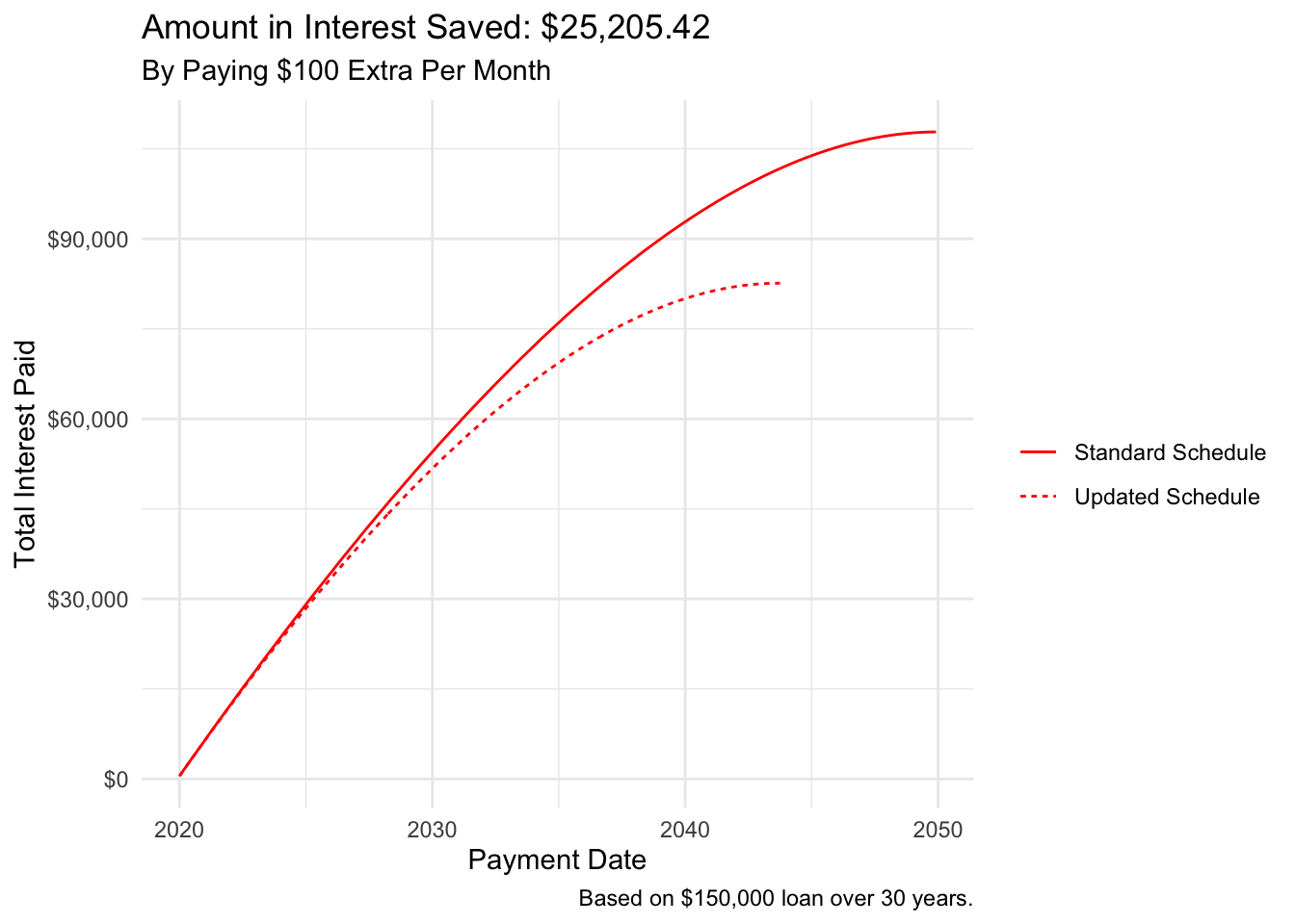
Spencer Schien
Senior Manager of Data & Analytics
This is my bio. There are many like it, but this one is mine.