Mapping Crime in Milwaukee
About a year ago in the fall of 2018, I stumbled across data.milwaukee.gov. Suffice it to say, as a certified Data Nerd who accesses publicly available data in both my day job and my free time, I was impressed with the quality of the resources being provided by a city the size of Milwaukee. Maybe I’m easily impressed because I’m overly pessimistic about the capacity of our major cities, but we’ll leave that for another time…
At the time, I was only just beginning to tread water in the R pool, and I thought it would be a fun / instructive challenge to try to come up with an interesting visual representing crime in Milwaukee. Specifically, I had a vision of facet wrapping a map of crimes in Milwaukee by some characteristic of the data. And with this exceedingly vague sense of direction, I was off!
Accessing the Data
The first step is getting the data into R. The code below will read the crime data in .csv format provided on the data portal.
It should be noted that the city’s data portal does provide API access, but this was beyond my awareness and abilities when I first completed this project.
library(tidyverse)
## ── Attaching packages ─────────────────────────────────────── tidyverse 1.3.1 ──
## ✓ ggplot2 3.3.5     ✓ purrr   0.3.4
## ✓ tibble  3.1.6     ✓ dplyr   1.0.7
## ✓ tidyr   1.1.4     ✓ stringr 1.4.0
## ✓ readr   2.1.1     ✓ forcats 0.5.1
## ── Conflicts ────────────────────────────────────────── tidyverse_conflicts() ──
## x dplyr::filter() masks stats::filter()
## x dplyr::lag()    masks stats::lag()
# FYI this file is over 600,000 observations

crime <- read_csv("https://data.milwaukee.gov/dataset/5a537f5c-10d7-40a2-9b93-3527a4c89fbd/resource/395db729-a30a-4e53-ab66-faeb5e1899c8/download/wibrarchive.csv")
## Rows: 772367 Columns: 24
## ── Column specification ────────────────────────────────────────────────────────
## Delimiter: ","
## chr   (3): IncidentNum, Location, WeaponUsed
## dbl  (20): ReportedYear, ReportedMonth, ALD, NSP, POLICE, TRACT, WARD, ZIP, ...
## dttm  (1): ReportedDateTime
##
## ℹ Use `spec()` to retrieve the full column specification for this data.
## ℹ Specify the column types or set `show_col_types = FALSE` to quiet this message.
Preparing Data for Visualization
Now that we have the data loaded into R, we can use the glimpse function to get a snapshot of the fields present in the data.
glimpse(crime)
## Rows: 772,367
## Columns: 24
## $ IncidentNum      <chr> "050450118", "050450120", "050450121", "050450123", "…
## $ ReportedDateTime <dttm> 2005-02-14 10:21:00, 2005-02-14 20:30:00, 2005-02-14…
## $ ReportedYear     <dbl> 2005, 2005, 2005, 2005, 2005, 2005, 2005, 2005, 2005,…
## $ ReportedMonth    <dbl> 2, 2, 2, 2, 2, 2, 2, 2, 2, 2, 2, 2, 2, 2, 2, 2, 2, 2,…
## $ Location         <chr> "2880 N MENOMONEE RIVER PK", "1300 W LAYTON AV", "483…
## $ WeaponUsed       <chr> NA, NA, NA, NA, NA, NA, NA, NA, NA, NA, NA, NA, NA, N…
## $ ALD              <dbl> 5, 13, 1, 7, 4, 6, 14, 8, 9, 10, NA, 7, 6, 14, 15, 15…
## $ NSP              <dbl> NA, NA, 2, 1, 14, 4, NA, NA, NA, 5, NA, 5, 4, NA, 11,…
## $ POLICE           <dbl> 7, 6, 7, 7, 3, 5, 6, 2, 4, 7, NA, 7, 5, 6, 3, 3, 2, 3…
## $ TRACT            <dbl> 5600, 21400, 2500, 2600, 13400, 4600, 18400, 19000, 1…
## $ WARD             <dbl> 85, 308, 51, 64, 197, 115, 247, 259, 5, 164, NA, 101,…
## $ ZIP              <dbl> 53222, 53221, 53209, 53209, 53208, 53206, 53207, 5321…
## $ RoughX           <dbl> 2524559, 2554308, 2544045, 2545350, 2546970, 2552718,…
## $ RoughY           <dbl> 395722.5, 356497.6, 409236.0, 406543.5, 385290.7, 402…
## $ Arson            <dbl> 0, 0, 0, 0, 0, 0, 0, 0, 0, 0, 0, 0, 0, 0, 0, 0, 0, 0,…
## $ AssaultOffense   <dbl> 0, 0, 0, 0, 0, 0, 0, 0, 0, 0, 0, 0, 0, 0, 0, 0, 0, 0,…
## $ Burglary         <dbl> 1, 0, 0, 0, 0, 0, 0, 0, 0, 0, 0, 1, 0, 0, 0, 0, 1, 0,…
## $ CriminalDamage   <dbl> 0, 0, 0, 0, 0, 0, 1, 0, 0, 0, 0, 0, 0, 0, 0, 0, 0, 0,…
## $ Homicide         <dbl> 0, 0, 0, 0, 0, 0, 0, 0, 0, 0, 0, 0, 0, 0, 0, 0, 0, 0,…
## $ LockedVehicle    <dbl> 0, 0, 0, 0, 0, 0, 0, 0, 0, 0, 0, 0, 0, 0, 0, 1, 0, 0,…
## $ Robbery          <dbl> 0, 0, 0, 0, 0, 1, 0, 0, 0, 0, 1, 0, 0, 0, 0, 0, 0, 0,…
## $ SexOffense       <dbl> 0, 0, 0, 0, 0, 0, 0, 0, 0, 0, 0, 0, 0, 0, 0, 0, 0, 0,…
## $ Theft            <dbl> 0, 1, 1, 1, 1, 0, 0, 0, 1, 1, 0, 0, 1, 1, 1, 0, 0, 1,…
## $ VehicleTheft     <dbl> 0, 0, 0, 0, 0, 0, 0, 1, 0, 0, 0, 0, 0, 0, 0, 0, 0, 0,…
Given my stated intention of creating a faceted map, the first set of fields I’m looking for are those that provide some sort of location information, and as luck would have it, the city provides this data in the form of RoughX and RoughY. Without coordinates, the only way I knew to obtain plottable coordinates was to access the Google API and retrieve lat-long from physical address. Google’s API sets a limit, though, and at nearly 700K observations, this data exceeded that limit. If that was the route I had to take, it would have complicated the process.
Since we are fortunate enough to already have the coordinates, our next step is to coerce the data into a simple features object using the sf package. The greatest difficulty I had with this step was determining what Coordinate Reference System the city was using to plot these crimes–little did I know that the sf package also has a function (st_crs) to handle this task in a single line of code. So I’ll just consider the weeks (yes, this held me up for weeks until a kind user on Reddit pointed me in the right direction) I spent stuck on this chunk as a very hard earned lesson.
library(sf)
## Linking to GEOS 3.8.1, GDAL 3.2.1, PROJ 7.2.1; sf_use_s2() is TRUE
# cleaning data for mapping ====

crime_location <- crime %>%
  filter(!is.na(RoughX) & !is.na(RoughY)) %>%
  st_as_sf(coords = c("RoughX", "RoughY"), crs = 32054)
Now we have our crime data converted to a simple features object. If we want to map onto some representation of the city of Milwaukee–which we do–we need to also import those shapefiles and align everything to the same CRS.
# Shapefiles can be found online
# or I have a repo here: https://github.com/Pecners/shapefiles
# Note that you will need all files located in a single folder,
# and you can load it with this call

neighb <- read_sf("milwaukee_neighborhood/neighborhood.shp")

# align to the same CRS
crime_neighb <- st_transform(crime_location, crs = st_crs(neighb))
And just like that, we have all the data we need in a simple features format! We just need to shift gears here and do a bit a ordinary data tidying.
With our stated goal of faceting by a certain characteristic, one immediately evident possibility is to choose the type of crime as the facet variable. In order to facet a plot by the type of crime, though, we will need to bring all of the crimes under a single variable, as each separate crime is currently under a wide dummie format.
To clean this up, I chose to follow the tidyverse conventions and use gather(). I also filtered the data to only include the year 2018–this is both to reduce over plotting of points, and to ease the data manipulation.
These next few chunks can be a bit processor-heavy and take a while to run.
# this chunk takes a while
crime_neighb <- crime_neighb %>%
  filter(ReportedYear == 2021) %>%
  gather("Crime", "yn", -c(1:12, 23)) %>%
  # remove dummie `no` observations
  filter(yn != 0)

# this chunk takes a while longer
crime_neighb <- st_intersection(neighb, crime_neighb)
## Warning: attribute variables are assumed to be spatially constant throughout all
## geometries
Whew, we’re really sweating after those chunks! I’m sure this still isn’t optimized very well (I don’t even want to know what data.table adherents would have to say), but it works! Or at least, we think it will work. There’s only one way to know for sure, and that’s to finally get to producing the map.
The final package we will need is the tmap package that follows the grammar of graphics and makes it fairly simple to produce highly customizable plots using spatial data.
library(tmap)
## Warning: multiple methods tables found for 'direction'
## Warning: multiple methods tables found for 'gridDistance'
# make the map ====

# add the neighborhood data aesthetic
tm_shape(neighb) +
  # add polygon layer with borders set to transparent
  # this plots the grey city outline
  tm_polygons(border.alpha = 0) +
  # add the crime data aesthetic
 tm_shape(crime_neighb) +
  # add dot layer with 0.5 alpha to show overlap
  tm_dots(col = "red", alpha = 0.5) +
  # facet by our gathered `Crime` variable
  # free.coords = FALSE keeps each facet the same zoom
 tm_facets(by = "Crime", free.coords = FALSE) +
 tm_layout(main.title = "Reported Crimes in Milwaukee, 2021")
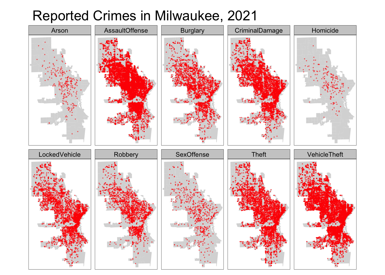
And there we have it! As I’ve tried to intimate throughout this post, I recognize that this might not be the optimal or most rigorous project of its kind, but I hope it is an instructive example for rapid prototyping from concept to minimal deliverable.
Any questions, comments, or suggestions are welcome–just shoot me an email.