Full Case Study Documentation
Introduction
Purpose
The purpose of this project is to provide a recommendation for the optimal allocation of development staff at Shocjin Nonprofit sites to either corporation/foundation giving or to Giving Society (GS) giving. Based on the given survey data, it is implied that the numbers represent a stable state (i.e. the number of engagements and rate of success will not diminish with time as the site cycles through the local corporations or other giving populations).
To arrive at a recommendation, the following process will be followed:
- Simulate annual giving for both corporations and GS. This will create two dataframes in which each observation represents a gift. Each will also simulate the number of years the gift will be extended. Therefore, each dataframe will represent total commitments from a single year, including those that will be paid in the given year and those that will be anticipated in coming years.
- Wrap this simulation in a function so it can be used with
replicate()to run a Monte Carlo simulation for a given year. - Loop the simulation over multiple years to simulate giving trends extending beyond the typical life-cycle of a single year’s gifts. This method will allow the simulation to reach a stable state, where the additive influence of gifts accumulating and expiring has leveled off.
- Determine the range of giving that can be expected with 90% confidence during the stable state of giving for both groups.
- Make the recommendation that allows for an acceptable level of risk while still maintaining an adequate level of giving for each site.
Further Questions and Additional Data
This analysis and recommendation is based on distributions and probabilities of survey data, representing a 90% confidence interval. The accuracy of any simulations are therefore limited and would be enhanced with access to the raw data.
Questions:
- What impacts the distribution of the number of engagements per year? If it is a function of the size of the city’s population or economy, then more specific recommendations could be made to sites.
- Do we observe stable replacement of gifts over the years? This simulation assumes that the answer is yes – meaning there is not a point where the giving supply is “tapped out”, so to speak.
- What other forms of return does a Shocjin Nonprofit site receive from engagements with corporations or individuals through the Giving Society? This analysis is based solely on the financial return in terms of giving, but returns in the form of enhanced recruitment, partnerships that might reduce or distribute costs, etc. could be considered as well.
Modeling
1. Simulating the Data
First, we need to recreate a single year of giving for both corporate and GS giving. The code below simulates the appropriate number of engagements, the success rate of engagements, the distribution of gift sizes, and the distribution of gift extensions.
library(EnvStats) # for truncated distributions
library(tidyverse) # for data manipulation and visualization
library(scales) # for setting percentages and scales, specifically in visuals
library(ggbeeswarm) # for creating the violin-like dot plot
library(ggalt) # for dumbbell plot

# set seed to ensure reproducibility
set.seed(123)

# Randomly assign the number of new corporations engaged in the year
# based on a truncated normal distribution; sd is estimated to ensure full
# range shows up in the samples. Samples are rounded to the nearest
# integer so we don't have partial engagements.
new_cos <- round(rnormTrunc(1, mean = 20, sd = 10/6, min = 15, max = 25), 0)

# Assign the number of successes (i.e. gifts)
success_cos <- round(new_cos * .25, 0)

# Set up mean and sd for the lognormal distribution
# of gift sizes.  Both are estimates since real values
# weren't provided.
avg_cos <- mean(c(log(50000), log(1000000)))
stdev_cos <- log(((1000000) - (50000))/success_cos)

# Simulate single year gifts by sampling a truncated lognormal
# distribution based on the values calculated above.
dis_cos <- rlnormTrunc(success_cos, avg_cos, stdev_cos, min = 50000, max = 1000000)

# Make a dataframe out of this vector, adding the simulation index `N`,
# the years each gift will be repeated `years_extended`, and the total
# commitments represented by this year of giving `total_commitment`
dis_cos <- tibble(amount = dis_cos, N = 1, years_extended = rpois(success_cos, 2) + 1,
              total_commitment = amount * years_extended)
dis_cos
## # A tibble: 5 × 4
##    amount     N years_extended total_commitment
##     <dbl> <dbl>          <dbl>            <dbl>
## 1 529597.     1              3         1588790.
## 2 170353.     1              5          851766.
## 3 703527.     1              3         2110580.
## 4 836028.     1              3         2508083.
## 5  57346.     1              6          344074.
2. Wrapping in a Function
Next, we need to wrap this simulation in a function that will allow us to append sequential simulations to the same dataframe. This is achieved with the following code, which makes the same parameter assignments as above:
sim_cos <- function() {
  new_cos <- round(rnormTrunc(1, mean = 20, sd = 10/6, min = 15, max = 25), 0)
  success_cos <- round(new_cos * .25, 0)


  avg_cos <- mean(c(log(50000), log(1000000)))
  stdev_cos <- log(((1000000) - (50000))/success_cos)

  # Make a base assignment with `dis_cos`, then a secondary assignment
  # with `dis_cos1` that will be rewritten and appended to the base with
  # each iteration.
  if(is.null(dis_cos)) {
    dis_cos <- rlnormTrunc(success_cos, avg_cos, stdev_cos, min = 50000, max = 1000000)
    dis_cos <- tibble(amount = dis_cos, N = 1,
                      # `years_extended` set to follow Poisson distribution
                      years_extended = rpois(success_cos, 2) + 1,
                      total_commitment = amount * years_extended)
  } else {
    dis_cos1 <- rlnormTrunc(success_cos, avg_cos, stdev_cos, min = 50000, max = 1000000)
    dis_cos1 <- tibble(amount = dis_cos1, N = max(dis_cos$N) + 1,
                       years_extended = rpois(success_cos, 2) + 1,
                   total_commitment = amount * years_extended)
  }
  dis_cos <<- bind_rows(dis_cos, dis_cos1)
}

# Test the function.  Output confirms that simulation is
# successful and appended to the base.
test_sim <- sim_cos()
test_sim
## # A tibble: 10 × 4
##     amount     N years_extended total_commitment
##      <dbl> <dbl>          <dbl>            <dbl>
##  1 529597.     1              3         1588790.
##  2 170353.     1              5          851766.
##  3 703527.     1              3         2110580.
##  4 836028.     1              3         2508083.
##  5  57346.     1              6          344074.
##  6 380189.     2              1          380189.
##  7 277811.     2              2          555622.
##  8  68134.     2              6          408802.
##  9 739936.     2              5         3699679.
## 10 104654.     2              4          418618.
The above dataframe represents two simulations of a single year of giving for corporations. So, we have our function working. Now we can run it for real to simulate a single year of giving one thousand times (or more, if we wanted).
# Clear the old `dis_cos` value from the envirnment
# so we can start anew.
rm(dis_cos)

# initialize the assignments needed by the function
dis_cos <- dis_cos1 <- NULL

# Use `replicate()` for the Monte Carlo simulation
replicate(1000, sim_cos())
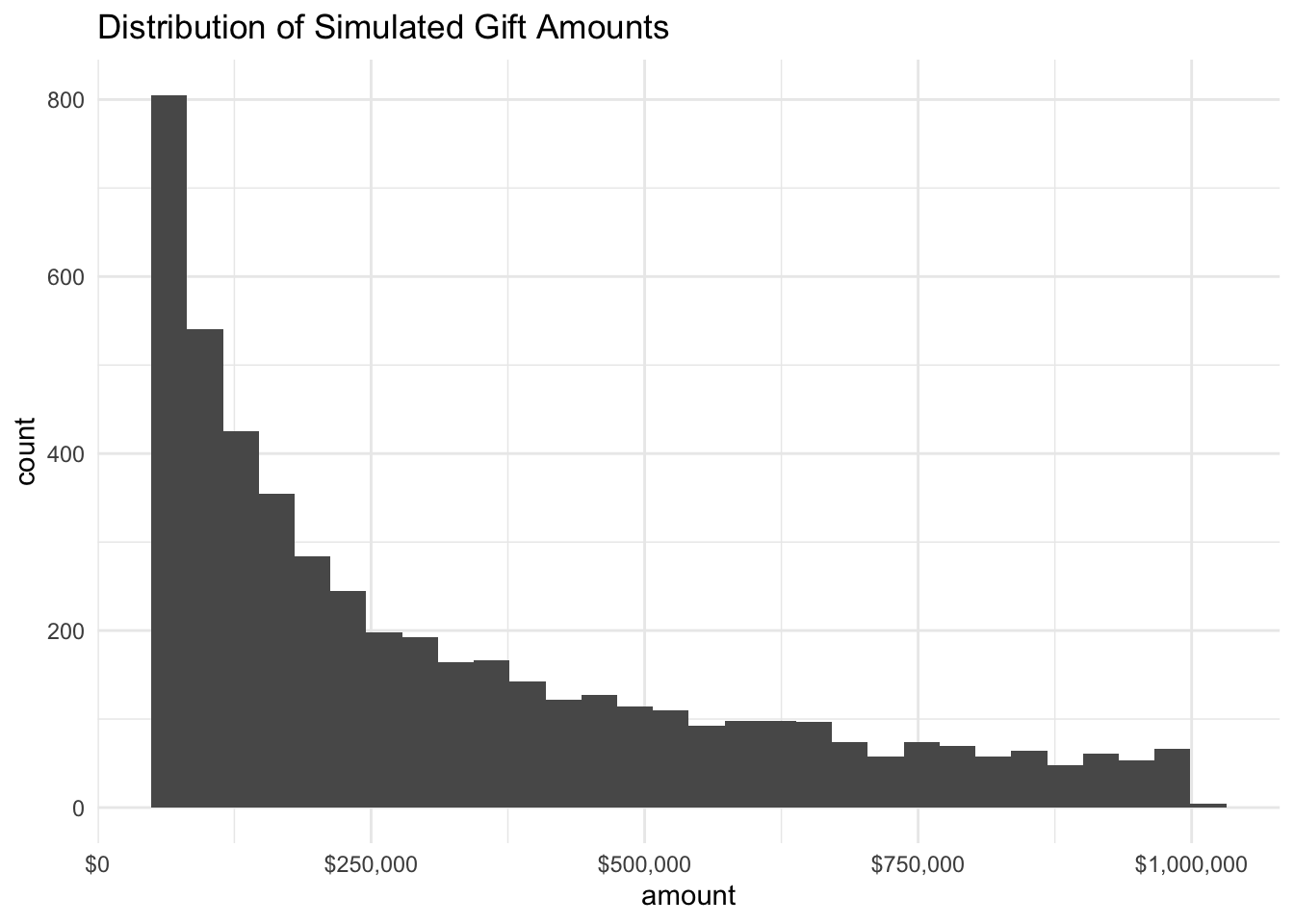
Now to make a quick inspection of the data we just simulated, we can review the distribution of both the gift sizes and the number of years the gifts are extended.
dis_cos %>%
  ggplot(aes(amount)) +
  geom_histogram() +
  theme_minimal() +
  scale_x_continuous(labels = dollar) +
  labs(title = "Distribution of Simulated Gift Amounts")
dis_cos %>%
  ggplot(aes(years_extended)) +
  geom_histogram() +
  theme_minimal() +
  scale_x_continuous(breaks = c(seq(1, max(dis_cos$years_extended), by = 1))) +
  labs(title = "Distribution of Simulated Number of Years Extended")
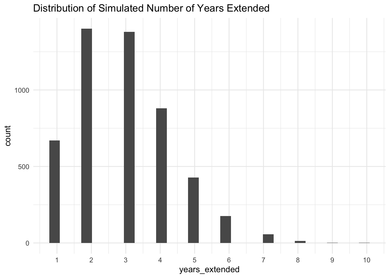
Ranges and distributions look as-expected, so we can move on to the next step which is to loop this simulation over multiple years.
3. Loop over Multiple Years
For this loop, we will edit the function slightly to add columns tracking the giving over each year.
# rewritten function with additional columns
sim_cos <- function() {
  new_cos <- round(rnormTrunc(1, mean = 20, sd = 10/6, min = 15, max = 25), 0)
  success_cos <- round(new_cos * .25, 0)

  avg_cos <- mean(c(log(50000), log(1000000)))
  stdev_cos <- log(((1000000) - (50000))/success_cos)

  if(is.null(dis_cos)) {
    dis_cos <- rlnormTrunc(success_cos, avg_cos, stdev_cos, min = 50000, max = 1000000)
    dis_cos <- tibble(amount = dis_cos, N = 1,
                      years_extended = rpois(success_cos, 2) + 1,
                  total_commitment = amount * years_extended)
  } else {
    dis_cos1 <- rlnormTrunc(success_cos, avg_cos, stdev_cos, min = 50000, max = 1000000)
    dis_cos1 <- tibble(amount = dis_cos1, N = max(dis_cos$N) + 1,
                       years_extended = rpois(success_cos, 2) + 1,
                   total_commitment = amount * years_extended)
  }
  dis_cos <<- bind_rows(dis_cos, dis_cos1) %>%
    # add the columns to track giving over the years
    mutate(start_year = i,
           year_1 = ifelse(start_year <= 0 & start_year + years_extended >= 1, amount, 0),
           year_2 = ifelse(start_year <= 1 & start_year + years_extended >= 2, amount, 0),
           year_3 = ifelse(start_year <= 2 & start_year + years_extended >= 3, amount, 0),
           year_4 = ifelse(start_year <= 3 & start_year + years_extended >= 4, amount, 0),
           year_5 = ifelse(start_year <= 4 & start_year + years_extended >= 5, amount, 0),
           year_6 = ifelse(start_year <= 5 & start_year + years_extended >= 6, amount, 0),
           year_7 = ifelse(start_year <= 6 & start_year + years_extended >= 7, amount, 0),
           year_8 = ifelse(start_year <= 7 & start_year + years_extended >= 8, amount, 0),
           year_9 = ifelse(start_year <= 8 & start_year + years_extended >= 9, amount, 0),
           year_10 = ifelse(start_year <= 9 & start_year + years_extended >= 10, amount, 0))
}

# Initialize new value that will be the full dataframe
cos <- NULL

# loop over 10 years starting with 0
# to facilitate addition of `years_extended`
for(i in 0:9) {

  # re-initialize inside the loop
  dis_cos <- dis_cos1 <- NULL

  # Monte Carlo
  replicate(1000, sim_cos())

  # Append each round of simulations
  cos <- bind_rows(cos, dis_cos)
}
The result of the above code is a dataframe that represents one thousand simulations of a single year of corporate giving repeated sequentially for 10 years (i.e. 10,000 year-giving simulations). The dataframe has the following attributes:
glimpse(cos)
## Rows: 49,935
## Columns: 15
## $ amount           <dbl> 205220.94, 439211.78, 225424.40, 680839.15, 362518.02…
## $ N                <dbl> 1, 1, 1, 1, 1, 1, 2, 2, 2, 2, 2, 3, 3, 3, 3, 3, 4, 4,…
## $ years_extended   <dbl> 6, 4, 2, 2, 2, 3, 3, 2, 4, 1, 3, 3, 2, 1, 3, 4, 3, 6,…
## $ total_commitment <dbl> 1231325.65, 1756847.13, 450848.81, 1361678.30, 725036…
## $ start_year       <int> 0, 0, 0, 0, 0, 0, 0, 0, 0, 0, 0, 0, 0, 0, 0, 0, 0, 0,…
## $ year_1           <dbl> 205220.94, 439211.78, 225424.40, 680839.15, 362518.02…
## $ year_2           <dbl> 205220.94, 439211.78, 225424.40, 680839.15, 362518.02…
## $ year_3           <dbl> 205220.94, 439211.78, 0.00, 0.00, 0.00, 242954.82, 24…
## $ year_4           <dbl> 205220.94, 439211.78, 0.00, 0.00, 0.00, 0.00, 0.00, 0…
## $ year_5           <dbl> 205220.9, 0.0, 0.0, 0.0, 0.0, 0.0, 0.0, 0.0, 0.0, 0.0…
## $ year_6           <dbl> 205220.9, 0.0, 0.0, 0.0, 0.0, 0.0, 0.0, 0.0, 0.0, 0.0…
## $ year_7           <dbl> 0, 0, 0, 0, 0, 0, 0, 0, 0, 0, 0, 0, 0, 0, 0, 0, 0, 0,…
## $ year_8           <dbl> 0, 0, 0, 0, 0, 0, 0, 0, 0, 0, 0, 0, 0, 0, 0, 0, 0, 0,…
## $ year_9           <dbl> 0, 0, 0, 0, 0, 0, 0, 0, 0, 0, 0, 0, 0, 0, 0, 0, 0, 0,…
## $ year_10          <dbl> 0, 0, 0, 0, 0, 0, 0, 0, 0, 0, 0, 0, 0, 0, 0, 0, 0, 0,…
4. Determine Expected Range
Now to the good stuff – visualizing and analyzing our full range of simulated data to come up with expected giving ranges.
# Before viz, we need to tidy the data a bit.
# Below code transforms from wide to long format,
# Which is easier to plot.  Also calculates annual
# giving totals for each simulation.
cos_years <- cos %>%
  group_by(N) %>%
  summarise_at(vars(year_1:year_10), sum) %>%
  pivot_longer(cols = c(2:11), names_to = "year", values_to = "year_amount") %>%
  modify_at("year", fct_relevel, levels = c("year_1",
                                            "year_2",
                                            "year_3",
                                            "year_4",
                                            "year_5",
                                            "year_6",
                                            "year_7",
                                            "year_8",
                                            "year_9",
                                            "year_10")) %>%
  group_by(N, year) %>%
  summarise(year_total = sum(year_amount)) %>%
  mutate(cum_total = cumsum(year_total),
         category = "cos")


# Plot the annual giving for each simulation.
cos_years %>%
  ggplot(aes(year, year_total)) +
  geom_line(aes(group = N), alpha = 0.5) +
  theme_minimal() +
  scale_y_continuous(labels = dollar)+
  expand_limits(y = 0) +
  labs(title = "1,000 10-Year Corporate Giving Simulations",
       y = "Total Gifts Received",
       x = "Year of Simulation")
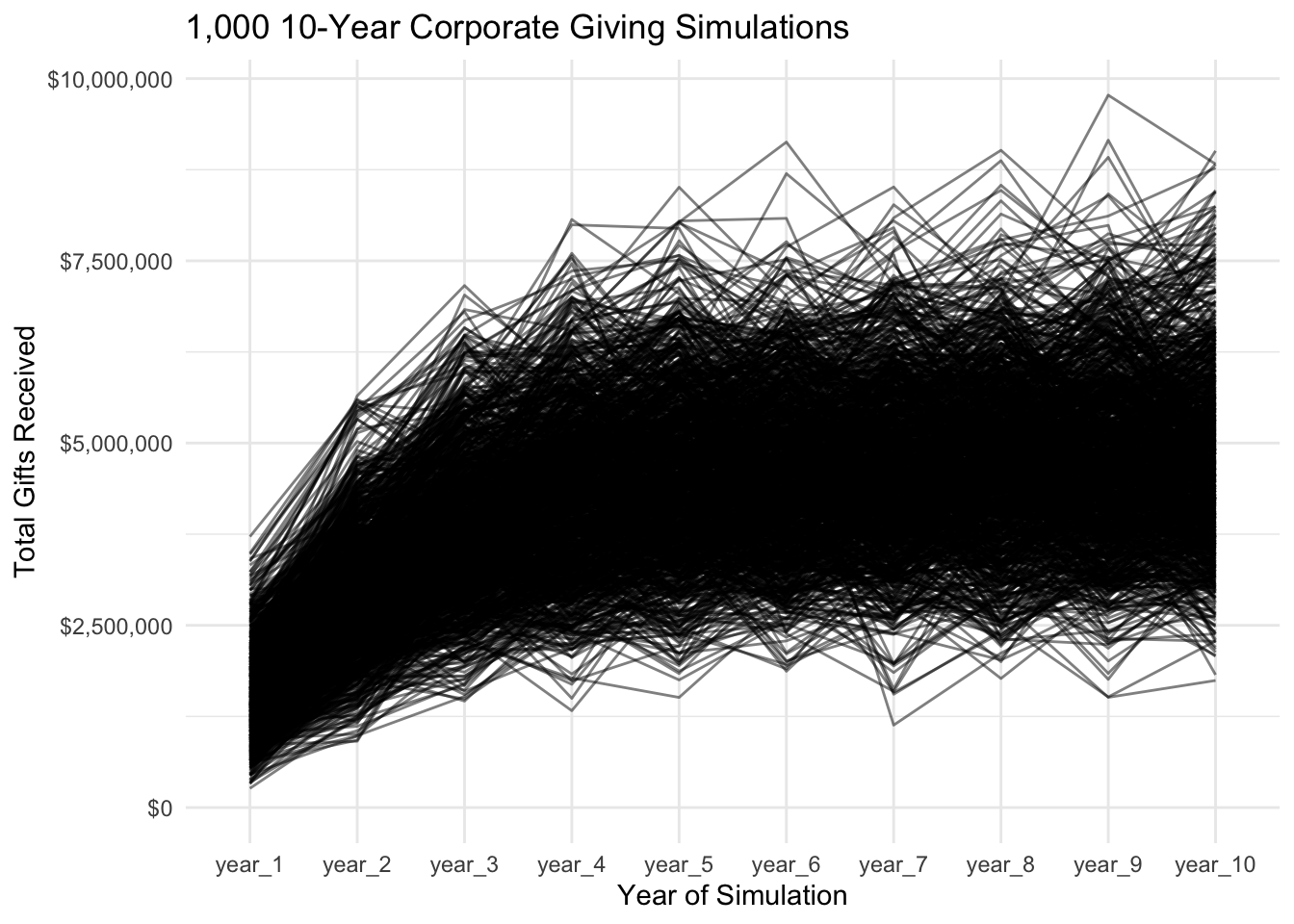
As is evident from this visual, giving does in fact reach a more stable state by year_10, and it is from this stable state that we will take our estimate of expected corporate giving. To do so, we will calculate the 90% confidence interval for years six through ten.
# Filter data for years 6 - 10
cos_latter <- cos %>%
  group_by(N) %>%
  summarise_at(vars(year_1:year_10), sum) %>%
  pivot_longer(cols = c(2:11), names_to = "year", values_to = "year_amount") %>%
  modify_at("year", fct_relevel, levels = c("year_1",
                                            "year_2",
                                            "year_3",
                                            "year_4",
                                            "year_5",
                                            "year_6",
                                            "year_7",
                                            "year_8",
                                            "year_9",
                                            "year_10")) %>%
  mutate(year = as.numeric(year)) %>%
  filter(year > 5)

# Will calculate the CI at the end to avoid loading
# Rmisc package which causes conflicts
Adding Giving Society Simulation
Now it’s time to run the same analysis over the GS giving. The below code does the same as we did above for corporate giving:
sim_GS <- function() {
new_GS <- round(rnormTrunc(1, mean = 350, sd = 300/6, min = 200, max = 500), 0)
success <- round(new_GS * .5, 0)
min <- 5000
max <- 50000
avg <- mean(c(log(5000), log(50000)))
stdev <- log(((50000) - (5000))/success)
if(is.null(dis)) {
dis <- rlnormTrunc(success, avg, stdev, min = min, max = max)
dis <- tibble(amount = dis, N = 1, years_extended = sample(c(1, 2, 3),
size = success,
prob = c(.5, .4, .1),
replace = TRUE),
total_commitment = amount * years_extended)
} else {
dis1 <- rlnormTrunc(success, avg, stdev, min = min, max = max)
dis1 <- tibble(amount = dis1, N = max(dis$N) + 1,
years_extended = sample(c(1, 2, 3),
size = success,
prob = c(.5, .4, .1),
replace = TRUE),
total_commitment = amount * years_extended)
}
dis <<- bind_rows(dis, dis1) %>%
mutate(start_year = i,
year_1 = ifelse(start_year <= 0 & start_year + years_extended >= 1, amount, 0),
year_2 = ifelse(start_year <= 1 & start_year + years_extended >= 2, amount, 0),
year_3 = ifelse(start_year <= 2 & start_year + years_extended >= 3, amount, 0),
year_4 = ifelse(start_year <= 3 & start_year + years_extended >= 4, amount, 0),
year_5 = ifelse(start_year <= 4 & start_year + years_extended >= 5, amount, 0),
year_6 = ifelse(start_year <= 5 & start_year + years_extended >= 6, amount, 0),
year_7 = ifelse(start_year <= 6 & start_year + years_extended >= 7, amount, 0),
year_8 = ifelse(start_year <= 7 & start_year + years_extended >= 8, amount, 0),
year_9 = ifelse(start_year <= 8 & start_year + years_extended >= 9, amount, 0),
year_10 = ifelse(start_year <= 9 & start_year + years_extended >= 10, amount, 0))
}
GS <- NULL
for(i in 0:9) {
dis <- dis1 <- NULL
replicate(1000, sim_GS())
GS <- bind_rows(GS, dis)
}
GS_years <- GS %>%
group_by(N) %>%
summarise_at(vars(year_1:year_10), sum) %>%
pivot_longer(cols = c(2:11), names_to = "year", values_to = "year_amount") %>%
group_by(N, year) %>%
summarise(year_total = sum(year_amount)) %>%
mutate(cum_total = cumsum(year_total),
category = "GS") %>%
modify_at("year", fct_relevel, levels = c("year_1",
"year_2",
"year_3",
"year_4",
"year_5",
"year_6",
"year_7",
"year_8",
"year_9",
"year_10"))
GS_latter <- GS %>%
group_by(N) %>%
summarise_at(vars(year_1:year_10), sum) %>%
pivot_longer(cols = c(2:11), names_to = "year", values_to = "year_amount") %>%
modify_at("year", fct_relevel, levels = c("year_1",
"year_2",
"year_3",
"year_4",
"year_5",
"year_6",
"year_7",
"year_8",
"year_9",
"year_10")) %>%
mutate(year = as.numeric(year)) %>%
filter(year > 5)
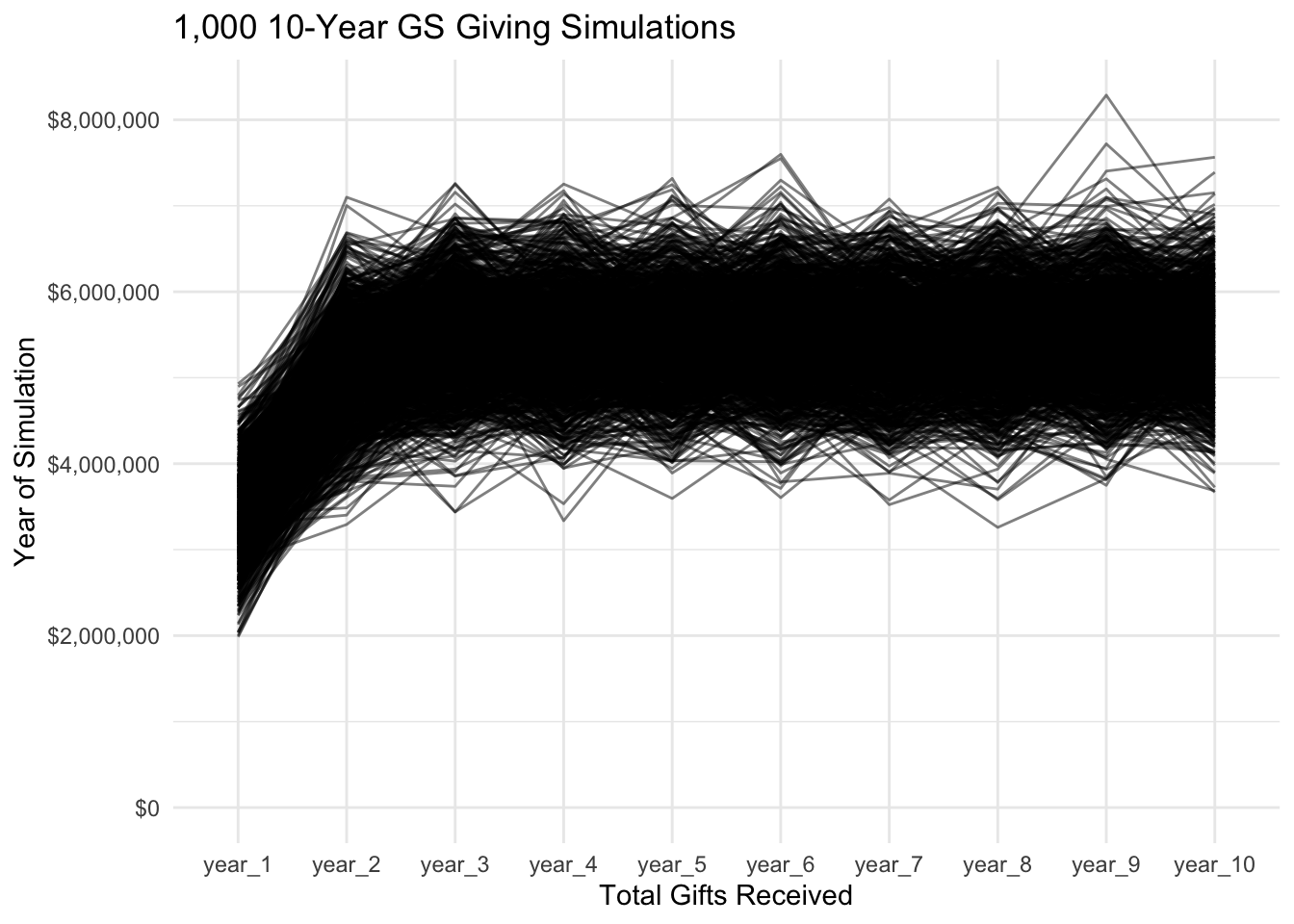
GS_years %>%
ggplot(aes(year, year_total)) +
geom_line(aes(group = N), alpha = .5) +
theme_minimal() +
scale_y_continuous(labels = dollar) +
expand_limits(y = 0) +
labs(title = "1,000 10-Year GS Giving Simulations",
x = "Total Gifts Received",
y = "Year of Simulation")
Analysis
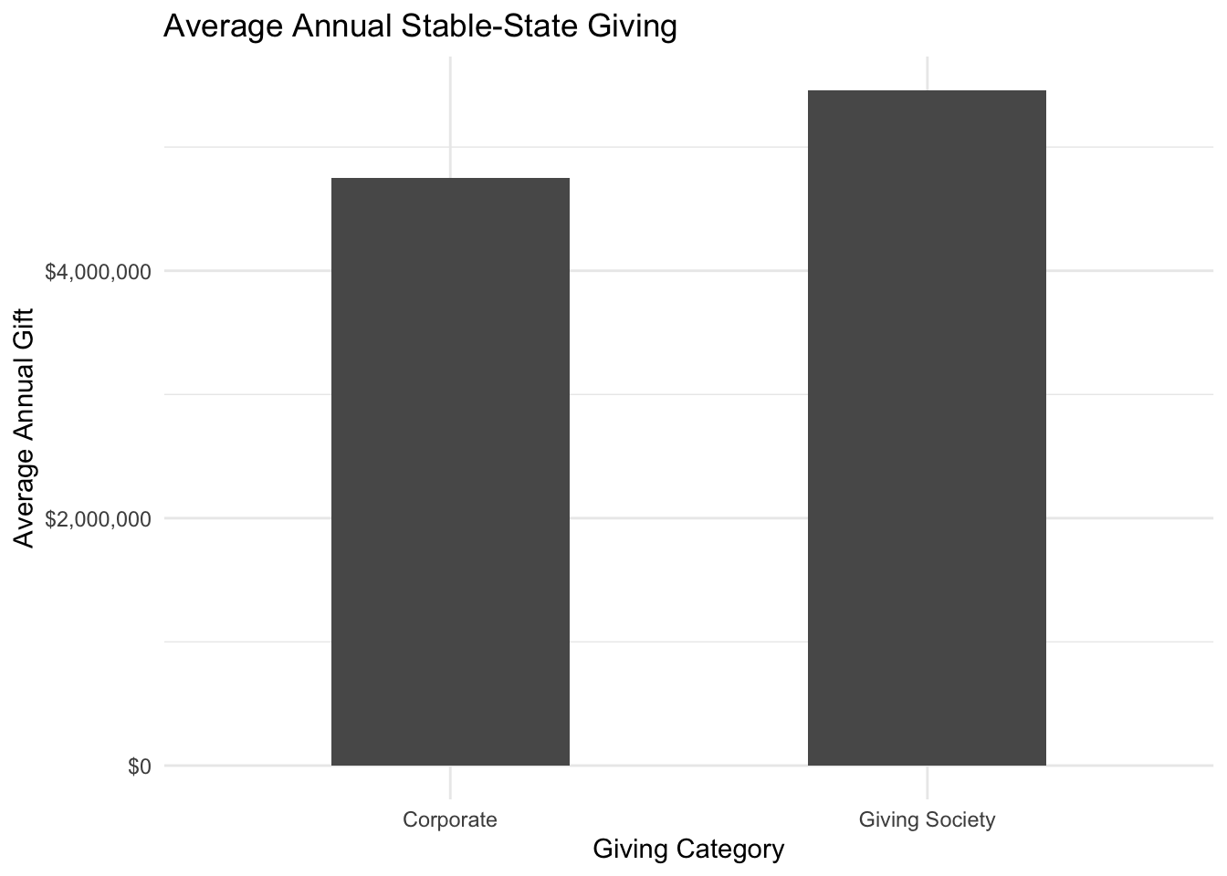
The visual below represents the average giving over this stable period.
cos_avg <- mean(cos_latter$year_amount)
GS_avg <- mean(GS_latter$year_amount)

avg_df <- tibble(category = c("Corporate", "Giving Society"),
                 amount = c(cos_avg, GS_avg))

avg_df %>%
  ggplot(aes(category, amount)) +
  geom_col(width = .5) +
  theme_minimal() +
  scale_y_continuous(labels = dollar) +
  labs(title = "Average Annual Stable-State Giving",
       x = "Giving Category",
       y = "Average Annual Gift")
This represents the 90% probability that the true mean will be represented within the span, which is a useful metric. However, we want to also mitigate risk (i.e. the possibility that total gifts will come in lower than expected).
As the 10-year line graphs demonstrated above, neither giving category will be expected to lose money once a stable state is reached (in initial simulations not represented here, corporate giving did show a potential for zero gifts in year_1). Therefore, the risk should be assessed in terms of the lowest potential return.
# define 95% range of data
quant_cos <- quantile(cos_latter$year_amount, c(.025, .975))
quant_GS <- quantile(GS_latter$year_amount, c(.025, .975))

# combine in a dataframe for visualization
quants_df <- tibble(Corporate = quant_cos, "Giving Society" = quant_GS) %>%
  pivot_longer(1:2, names_to = "category", values_to = "amount") %>%
  group_by(category) %>%
  summarise(xend = min(amount),
            x = max(amount))


quants_df %>%
  ggplot(aes(y = "")) +
  geom_dumbbell(aes(xend = xend, x = x), size_x = 3, size_xend = 3) +
  geom_vline(data = avg_df, aes(xintercept = amount), linetype = 3) +
  geom_text(y = .7, x = avg_df$amount + avg_df$amount*.1,
           label = paste("Average Annual Giving:", dollar(avg_df$amount), sep = "\n"),
           size = 2) +
  facet_wrap(~ category) +
  theme_minimal() +
  scale_x_continuous(labels = dollar, breaks = c(0, 2500000, 5000000, 7500000)) +
  expand_limits(x = 0) +
  labs(title = "Expected Range of Giving",
         subtitle = "85% probability that giving will fall within this range",
         x = "",
         y = "") +
  coord_flip()
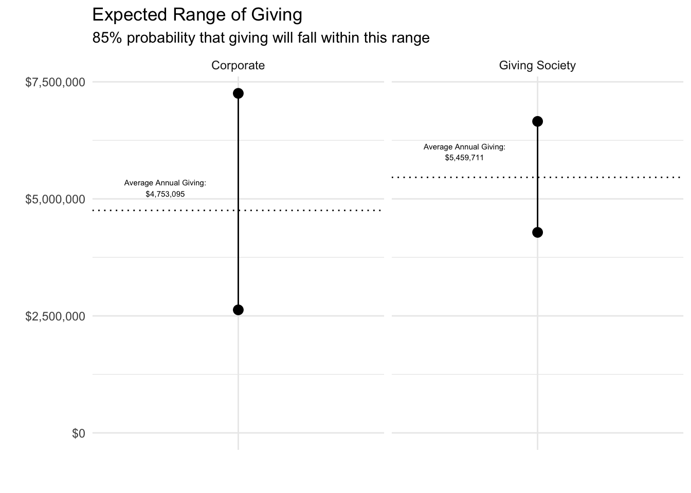
The above visual gives the simulated 95% ranges from the stable-giving period for both giving categories. Since the original data from which this simulation was formulated represented a 90% confidence interval, that will translate through the simulations. Therefore, we can expect that there is an 85% chance that giving will fall in the ranges depicted above, which means there is a 15% chance that giving will fall outside of those ranges – 7.5% for both higher and lower giving.
With this in mind, we can define the risk of each category as the giving level at which there is a 7.5% chance giving will fall below that level.
The Recommendation
Finally, we are at a point to define the risk of different distributions of development focus between corporate giving and GS giving.
The code below determine for each simulation whether the total giving for the year (the sum of corporate and GS giving) is less than the average annual
avg <- (cos_avg + GS_avg)
est_loss_stable <- function(t, w) {
total <- t
weight <- w * total
break_even <- t / 2 * avg
all_years_stable <- bind_rows(GS_years, cos_years) %>%
select(-cum_total) %>%
filter(as.numeric(year) > 5) %>%
pivot_wider(names_from = category, values_from = year_total) %>%
mutate(loss = ifelse(
break_even > (GS * (weight) + cos * (total - weight)), 1, 0
))
est_df_stable <- tibble(total = t, weight = w,
loss_prob = mean(all_years_stable$loss))
est_df_stable
}
est_loss_startup <- function(t, w) {
total <- t
weight <- w * total
break_even <- t / 2 * avg
all_years_startup <- bind_rows(GS_years, cos_years) %>%
select(-cum_total) %>%
filter(as.numeric(year) < 6) %>%
pivot_wider(names_from = category, values_from = year_total) %>%
mutate(loss = ifelse(
break_even > (GS * (weight) + cos * (total - weight)), 1, 0
))
est_df_startup <<- tibble(total = t, weight = w,
loss_prob = mean(all_years_startup$loss))
est_df_startup
}
est_table <- expand_grid(t = 1:5, w = seq(from = 0, to = 1, by = .05))
est_df_stable <- map2_df(est_table$t, est_table$w, est_loss_stable)
est_df_startup <- map2_df(est_table$t, est_table$w, est_loss_startup)
est_df_stable %>%
ggplot(aes(weight, loss_prob, group = total)) +
geom_line() +
theme_minimal() +
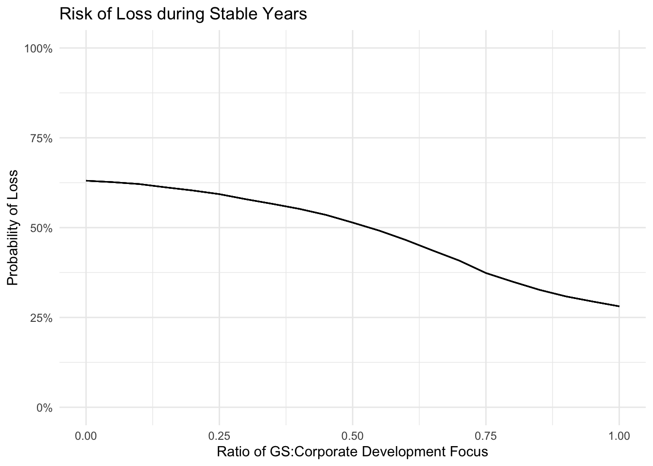
labs(x = "Ratio of GS:Corporate Development Focus",
y = "Probability of Loss",
title = "Risk of Loss during Stable Years") +
scale_y_continuous(labels = percent, limits = c(0, 1))
est_df_startup %>%
  ggplot(aes(weight, loss_prob, group = total)) +
  geom_line() +
  theme_minimal() +
  labs(x = "Ratio of GS:Corporate Development Focus",
       y = "Probability of Loss",
       title = "Risk of Loss during Start-up Years") +
  scale_y_continuous(labels = percent, limits = c(0, 1))
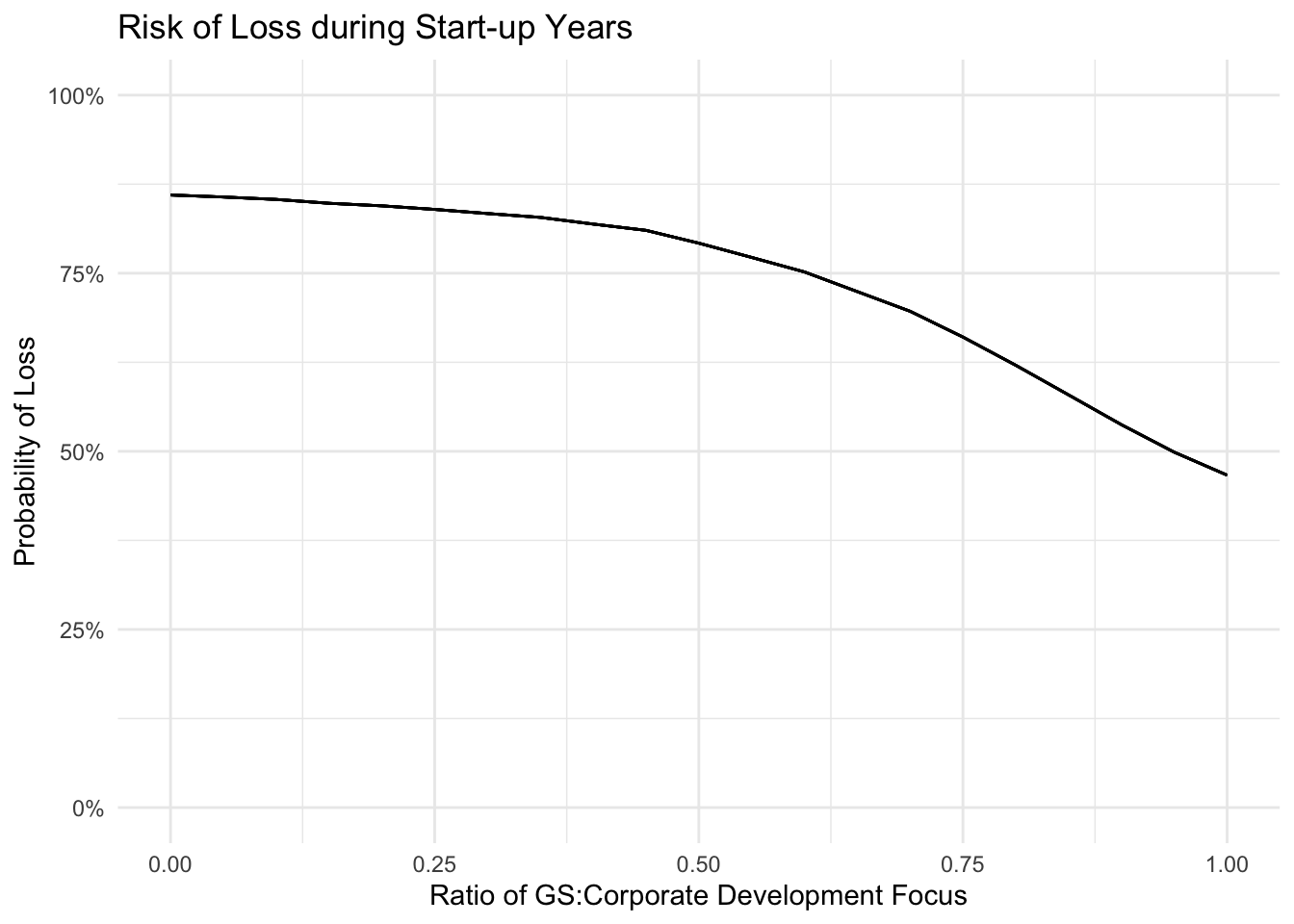
Figure 1: Loss here defined as any annual giving total less than the expected average given an equal distribution of focus between Giving Society and Corporate giving.
Based on this model, the optimal distribution of development staff would maximize focus on Giving Society giving, especially in startup years (i.e. first years of implementation for both types of giving). The level to which it is maximized should be determined by the non-monetary value of the corporate engagements.
Spencer Schien
Senior Manager of Data & Analytics
This is my bio. There are many like it, but this one is mine.