Spatial Analysis in Support of Fund Development
Introduction
This post describes a use case for R in support of fund development activities at a nonprofit, specifically using spatial analysis to make a case for funding. I have everything organized as a case study very similar to data requests I frequently receive.
The post will walk through the following steps:
- Find and plot spatial data for city and other geometries (e.g. neighborhoods)
- Create a spatial polygon from scratch to add to existing geometries
- Geocode points from addresses
- Perform spatial operations to determine if points fall within polygons or are within distance
xof polygons - Produce a final visualization in support of the analysis
Case Study
Many foundations that fund nonprofits have their own priorities they’re trying to advance. One such priority is often related to place, such as specific cities, ZIP codes, or even neighborhoods within a city. In fact, these foundations might limit funding to organizations that can prove they serve communities located in those places. It is therefore important to be able to identify the location of your organization’s stakeholders.
The Request
You work at a nonprofit organization in Milwaukee, Wisconsin that supports K-12 schools in the city. Your organization is submitting a grant application to the Fake Foundation, and your fund development team has asked you to provide some data that will help them make a case for funding.
The Fake Foundation is focused on three specific neighborhoods in Milwaukee, so the request is for data on which schools you support that are located in those three neighborhood.
The three neighborhoods are:
- Havenwoods
- Thurston Woods
- Westlawn
Your Data
First things first, let’s get a handle on where these three neighborhoods are within the city. To do this, we will need spatial data for the city as well as the individual neighborhoods. For a city like Milwaukee, there are officially-recognized neighborhood boundaries, and the city provides shapefiles for both general city limits as well as individual neighborhoods.
If you’d like to follow along with my code, you can download the neighborhood shapefile here, and you can download the city limits shapefile here. Otherwise, you can substitute your own spatial geometries.
.shp file, as below.
We’ll be using the sf R package for our spatial manipulation operations, plus the tidyverse for general operations and visualization. The code below will load the data and plot the three neighborhoods on top of the city limits, giving us a general idea of where the Fake Foundation’s focus is.
# Load packages we'll be using
library(tidyverse)
library(sf)
# Use `read_sf()` to read in shapefiles
# Neighborhood boundaries
nbds <- read_sf("data/milwaukee_neighborhood/neighborhood.shp") %>%
st_transform(crs = 4326)
# Milwaukee city limits
city <- read_sf("data/milwaukee_citylimit/citylimit.shp") %>%
st_transform(crs = 4326)
# Create a vector of the neighborhoods we want--
# all caps because that's how the data if formatted.
# Figure this out by inspecting the data with
# `glimpse(nbds)`, for instance.
focus <- c("HAVENWOODS",
"THURSTON WOODS",
"WESTLAWN")
# Filter full `nbds` data for our vector of focus
f_n <- nbds %>%
filter(NEIGHBORHD %in% focus)
# Plot the data, starting with citylimits
# then adding the neighborhoods
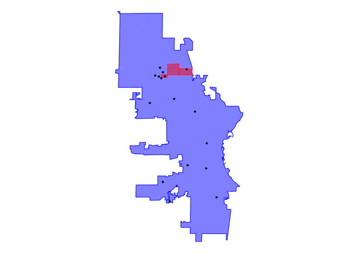
city %>%
ggplot() +
# Use fill, color, and alpha to easily distinguish between the
# different layers
geom_sf(fill = "blue", color = "blue", size = .5, alpha = .5) +
geom_sf(data = f_n, fill = "red", color = "red", size = .5, alpha = .5) +
# remove theme elements so it's easier to distinguish our polygons
theme_void()

As the plot shows, the focus neighborhoods are contiguous and on the north side of the city. It only looks like we have two neighborhoods plotted, though, when we listed three in our filter. We should have three different red polygons plotted, so what’s going on?
Once we inspect the filtered data contained in our f_n object, we can quickly see that there we only captured two neighborhoods: Havenwoods and Thurston Woods.
glimpse(f_n)
## Rows: 2
## Columns: 7
## $ AREA       <dbl> 23577729, 14911492
## $ PERIMETER  <dbl> 19528.03, 17302.98
## $ NBHDTEXT_  <dbl> 22, 100
## $ NBHDTEXT_I <dbl> 22, 100
## $ NEIGHBORHD <chr> "HAVENWOODS", "THURSTON WOODS"
## $ SYMBOL     <int> 4, 1
## $ geometry   <POLYGON [°]> POLYGON ((-87.96684 43.1322..., POLYGON ((-87.94598 43.1264…
The missing neighborhood is therefore Westlawn, which once we review our full neighborhood data in the nbds object, we see that Westlawn isn’t listed. Westlawn therefore is not an officially designated neighborhood, so we need to find its spatial data somewhere else.
It’s not uncommon to run into a scenario where an ad hoc boundary is needed or defined, requiring you to build the geometry yourself. Luckily, this is possible in R, but it does require a bit of legwork first.
Building a Custom Polygon
There are many ways to build a polygon in R, but one I prefer is to create a dataframe that contains separate columns for latitude and longitude. To get the coordinates, you can use Google Maps, but obviously you need some description of the boundaries. In our case, the Fake Foundation has provided images of their focus neighborhoods.
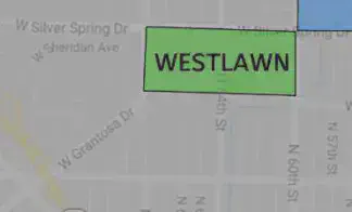
n polygon sides, you will need n+1 coordinate pairs.)
Now that we have our points that will define the boundary of the neighborhood, we need to turn it into a spatial object. The code below accomplishes this for us.
westlawn <- tibble(
  y = c(43.116010, 43.119315, 43.119457, 43.116010, 43.116010),
  x = c(-87.986190, -87.986190, -87.996060, -87.996060, -87.986190)
) %>%
  st_as_sf(., coords = c("x", "y"), crs = 4326) %>%
  mutate(NEIGHBORHD = "WESTLAWN") %>%
  group_by(NEIGHBORHD) %>%
  summarise() %>%
  st_cast(., to = "POLYGON")
Let’s dig into what’s going on here:
- The first step is inputting our coordinates into a dataframe (technically a tibble here)
- Next we convert our dataframe to a spatial object using
st_as_sf()- the
crsargument is important here, and it needs to be the same as the crs for our other neighborhoods (i.e.4326)
- the
- We create a column to match the name column of our
nbdsobject - By grouping by the neighborhood (of which there is only one) and sumarising a spatial object, we are combining the coordinates into a single observation or row
- We then cast this sumarised data to a polygon object
This isn’t super intuitive, I know, but it has accomplished our task. We can now add the Westlawn geometry to our two other neighborhoods and plot them again.
all_three <- bind_rows(f_n, westlawn)

p <- city %>%
  ggplot() +
  geom_sf(fill = "blue", color = "blue", size = .5, alpha = .5) +
  geom_sf(data = all_three, fill = "red", color = "red", size = .5, alpha = .5) +
  theme_void()

p

We did it! Now, you might be thinking something along the lines of, “Great, we plotted the neighborhoods, but I already knew where they were!” True, but the process of plotting the neighborhoods got us to a point where we have the specific spatial data we need in the format we need. Put another way, if we can plot the data, then we can join it with other data.
For our project here, we’re interested in joining this data with school location data. Our next step is to get that data into the appropriate spatial format.
Geocoding Addresses
The code below provides addresses for a sample of Milwaukee schools. Ultimately we will need spatial data for each school (i.e. latitude and longitude) – depending on where you’re getting your data, you might already have the necessary coordinates, in which case you can skip to the next section.
You can either use these sample addresses, or if you’re working with your own spatial geometries, you can use your own data or create a short vector of addresses yourself.
# Vector of address

school_address <- c("1712 S 32nd St Milwaukee WI 53215-2104",
                    "2320 W Burleigh St Milwaukee WI 53206-1751",
                    "357 E Howard Ave Milwaukee WI 53207-3923",
                    "4920 W Capitol Dr Milwaukee WI 53216-2321",
                    "6500 W Kinnickinnic River Pkwy Milwaukee WI 53219-3030",
                    "971 W Windlake Ave Milwaukee WI 53204-3822",
                    "3778 N 82nd St Milwaukee WI 53222-2999",
                    "609 N 8th St Milwaukee WI 53233-2405",
                    "4200 S 54th St Milwaukee WI 53220-3111",
                    "7000 W Florist Ave Milwaukee WI 53218",
                    "5440 N 64th St Milwaukee WI 53218-3020",
                    "5496 N 72nd St Milwaukee WI 53218-2820",
                    "5354 N 68th St Milwaukee WI 53218-2901",
                    "5760 N 67th St Milwaukee WI 53218-2307",
                    "5966 N 35th St Milwaukee WI 53209-4055",
                    "5460 N 64th St Milwaukee WI 53218-3020",
                    "5575 N 76th St Milwaukee WI 53218-2792")
Now that we have our addresses, we need to geocode them. To do so, we will be using the tidygeocoder package. As always, if you don’t already have this package installed, you’ll need to do so with install.packages("tidygeocoder").
# Load `tidygeocoder` so we can geocode the addresses

library(tidygeocoder)

# The data needs to be a dataframe for the
# `geocode()` function, so we will wrap our
# `school_address` vector in `tibble()`.

geocoded_schools <- tibble(
  school_address = school_address
) %>%
  geocode(address = school_address)

# Now examine output
head(geocoded_schools)
## # A tibble: 6 × 3
##   school_address                                           lat  long
##   <chr>                                                  <dbl> <dbl>
## 1 1712 S 32nd St Milwaukee WI 53215-2104                  43.0 -88.0
## 2 2320 W Burleigh St Milwaukee WI 53206-1751              43.1 -87.9
## 3 357 E Howard Ave Milwaukee WI 53207-3923                43.0 -87.9
## 4 4920 W Capitol Dr Milwaukee WI 53216-2321               43.1 -88.0
## 5 6500 W Kinnickinnic River Pkwy Milwaukee WI 53219-3030  43.0 -88.0
## 6 971 W Windlake Ave Milwaukee WI 53204-3822              43.0 -87.9
As we can see from our head() call output, the geocode() function has appended columns for latitude and longitude. We’re now ready to join this data with the neighborhood polygons.
Joining with Neighborhood Polygons
Just like we did with our custom Westlawn neighborhood geometry, we need to convert the actual coordinates to the appropriate sf object type.
# Keep in mind the CRS must be the same as our
# other geometries, which is 4326. Also, whereas
# for Westlawn we used `x` and `y` as our column
# names for the coordinates, we need to identify
# "long" and "lat" since that's what the
# `geocode()` function created.

f_geo_schools <- geocoded_schools %>%
  st_as_sf(coords = c("long", "lat"), crs = 4326)

# We can add a layer with the schools to our base plot
# we made earlier

p +
  geom_sf(data = f_geo_schools) +
  theme(plot.background = element_rect(fill = NA, color = NA))
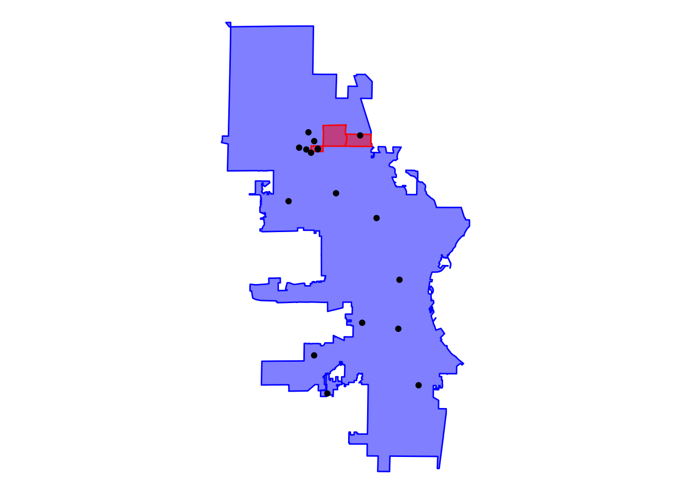
geom_sf() is smart enough to decide what kind of geom to apply given the type of spatial data. That is why we can layer geom_sf() calls on top of each other without specifying whether the geometry is a point, line, or polygon.
Based on this initial plot, we can see that nine of our schools aren’t in the vicinity of the neighborhoods, but seven schools are either in or near the neighborhoods. From here, we start to have a good idea of what we’ll be able to send to the fund development team.
Specifically, we can tell the team the number of schools located within the neighborhoods, and then we can bolster our case by including schools that are within a certain distance of these neighborhoods.
Spatial Operations
Our final step here is to determine two things. First, how many of these schools are within the neighborhoods, and second, how many schools are within a certain distance (e.g. half a mile).
For the first point, there are several ways we could get our answer, but let’s use the most straightforward. We want to know if the points (i.e. the schools) fall within the polygons (i.e. the neighborhoods). The st_contains() function will do exactly this for us, but an important thing to keep in mind is that these operations will compare all geometries against of one object against all geometries of another object.
For instance, our all_three object has three separate geometries, one for each neighborhood. f_geo_schools has 17 geometries, one for each school. Using st_contains() here will compare which schools fall within a single neighborhood one at a time, as if in a for loop. The object returned will then be a list of length three (for the three neighborhoods).
It is sometimes simpler to reduce the number of geometries that are being compared for this reason. In our scenario, we could reduce the number of neighborhoods by calling st_union(all_three), which would collapse the three polygons to a single geometry. The downside is that we wouldn’t then be able to easily identify which neighborhood contained the school.
So, we will maintain the three neighborhoods individually. The code below will create a list, and the list will contain an element for each neighborhood, and within each element, it will list the schools that fall within that neighborhood.
# Determine which schools are located within which neighborhoods
cross <- st_contains(all_three, f_geo_schools)

cross
## Sparse geometry binary predicate list of length 3, where the predicate
## was `contains'
##  1: (empty)
##  2: 15
##  3: 11, 16
As the output of cross shows us, there were no schools in the first neighborhood (Havenwoods), there was one in the second neighborhood, and there were two in the third for a total of three schools in the neighborhoods.
Next, we want to know what schools are located within a given distance of these neighborhoods. Half a mile is an intuitive distance for people to understand, plus it looks like there will be several more schools within a half-mile.
We can use the same st_contains() function call, but this time we’ll wrap the all_three object in a call to st_buffer(). st_buffer() will create a polygon around the object on which it is called, at a specified distance. The distance units are determined by the CRS, but for us here it’s meters. We will therefore need to convert half a mile to meters, which is about 805 meters.
# Which schools are within half a mile
cross_half_mi <- st_contains(st_buffer(all_three, 805), f_geo_schools)

cross_half_mi
## Sparse geometry binary predicate list of length 3, where the predicate
## was `contains'
##  1: 11, 14, 16
##  2: 15
##  3: 11, 12, 13, 14, 16
So, setting the buffer to half a mile, we have twice as many schools included.
Our Deliverable
We can now get back to the fund development team with hard data. Specifically, we can tell theme there are three schools located within the Fake Foundation’s focus neighborhoods, and there are three additional schools within half a mile. To support the data, we can also include a visualization.
The process of building this plot will provide us an example of alternatives to the st_contains() operation, too. Here’s the steps we will take:
- Combine the three geometries into a single one with
st_union() - Create the half-mile buffer around this unified geometry
- Call
st_intersection()to create a geometry of schools that intersect with the buffered neighborhoods - Plot the neighborhoods with the schools
st_intersection() because it effectively will perform the same function as st_contains() above, but it has the added benefit of returning a spatial object we can continue to plot or do other operations on.
schools_within <- st_intersection(
  f_geo_schools,
  st_buffer(
    st_union(all_three),
    805)
  )

all_three %>%
  ggplot() +
  geom_sf(fill = "red", color = "red", alpha = .5) +
  geom_sf_label(aes(label = str_to_title(NEIGHBORHD)),
                nudge_y = -.001, alpha = .75) +
  geom_sf(data = schools_within, alpha = .5) +
  theme_void()
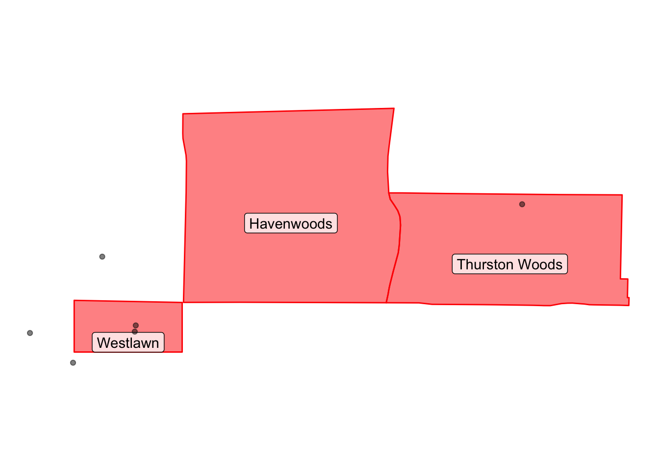
Conclusion
As I was writing this post, I had the thought that this might seem like a lot of work when you could have just looked up the few schools you knew to be in the neighborhood, and you’d be done. With this in mind, I want to close by pointing out the particular benefits of this methodology.
- This was an introduction to this sort of analysis. Depending on the questions you are trying to answer, you can quickly get much more complex in the analysis you are running.
- We were looking at limited neighborhoods and a small sample list of school addresses. In reality, this same analysis could scale very easily to include many more addresses, or it could be iterated on – for example, you could run this analysis and loop over a set of neighborhoods, zip codes, or other geometries of interest.
- If you already have R as part of your data stack (which I’m guessing you do since you’ve made it to the end of this post), this integrates seamlessly and can be further extended within your stack.
- On top of all this, you can produce publication quality visuals or reports to encapsulate your deliverable.
I hope this has been informative for you. As always, I welcome feedback or questions, so feel free to shoot me an email.
Spencer Schien
Senior Manager of Data & Analytics
This is my bio. There are many like it, but this one is mine.