LaTeX Tips for Rmd PDF Documents

Introduction

This post is a compilation of LaTeX tricks I’ve found useful in creating R Markdown PDF documents. In particular, these are techniques I had to research myself because they were not prominently documented in popular R Markdown resources. (Speaking of, I’ve found R Markdown: The Definitive Guide to be an excellent resource.)

For ease of use, here’s a list of techniques included in the post:

• Remove page numbers
• Add blank vertical space
• Change text size
• Highlight text
• Place a logo in header
• Place a logo in footer
• Increase table row height
• Dynamically create sections in code chunks

A Quick Note on LaTeX

Some of the examples below are lines of LaTeX that can be included within your R Markdown document body, and some require additions to the YAML. I want to provide a quick explanation of this before diving into the examples.

LaTeX documents are similar to HTML pages in that they begin with a section containing important data about document formatting and style, followed by the document body. In LaTeX, this first section is known as the preamble, but when working in R Markdown, the general term ‘header’ is often used. For instance, R Markdown templates will often come bundled with a header.tex document that contains specifications for the preamble.

The preamble basically sets the document defaults, such as page dimensions, font size, header/footer formatting, etc. It also specifies which LaTeX packages will be used in the document. This is important because, as with an R script, if there is a command you want to use that isn’t part of the base distribution of LaTeX, you need to include the package with your document. In such cases, you include the package in your preamble/header, which is what you see with the additions to the YAML in the examples below.

As with HTML, the document body contains a mixture of the actual copy content plus LaTeX commands that function in a similar way to HTML tags. When writing in R Markdown, you can include LaTeX code inline with your markdown text–you just need to be sure the necessary packages are loaded in the preamble.

Finally, as is the case with R, you do need to download the LaTeX packages you use. Fortunately for the R Markdown writer, this is done automatically when you knit a document that includes packages that aren’t already installed locally. In such cases, the production of the output document will take longer than usual, and you will see messages in the console that aren’t easily interpreted but that are regarding the download of necessary LaTeX packages. Assuming no errors, you document will still be output once the downloads are completed.

The Tips

Remove Page Numbers

Sometimes you’ll want to remove page numbers from a report. For me, this is most common when I create a one-page report. Page numbers can easily be removed by including \pagenumbering{gobble} in the header.

---
title: "Removing Page Numbers"
output: pdf_document
header-includes:
  - \pagenumbering{gobble}
---

## No Page Numbers

This document doesn't have page numbers.

Add Blank Vertical Space

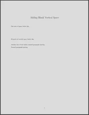
Adding blank vertical space can be accomplished with the \vsapce{lenght} command. This command takes a length argument, which accepts many different units. For instance, the example below shows how you can specify inches or pixels.

---
title: "Adding Blank Vertical Space"
output: pdf_document
---

One inch of space below this.

\vspace{1in}

20 pixels of verticle space below this.

\vspace{20px}

Another line of text before normal paragraph spacing.

Normal paragraph spacing.

Change Text Size

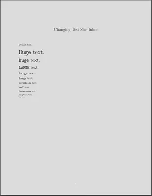
My most common use case for changing text size inline is when I want to have a very clear key take-away in a section that I want to jump off the page. Changing text size can be accomplished with a number of font size-modifier commands.

The import thing to remember with these commands is they start with the size modifier (e.g. \LARGE) and are closed with the \par tag.

---
title: "Changing Text Size Inline"
output: pdf_document
---

Default text.

\Huge `Huge` text.\par
\huge `huge` text.\par
\LARGE `LARGE` text.\par
\Large `Large` text.\par
\large `large` text.\par
\normalsize `normalsize` text.\par
\small `small` text.\par
\footnotesize `footnotesize` text.\par
\scriptsize `scriptsize` text.\par
\tiny `tiny` text.\par

Highlight Text

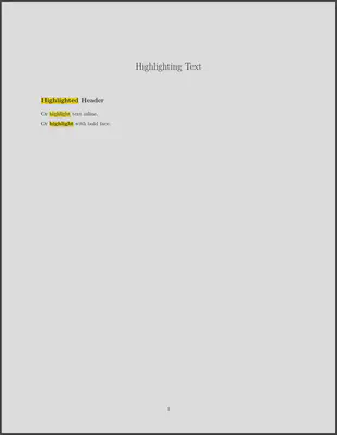
Similar to the use case I mentioned above for changing the text size, using highlighted text can help key points jump off the page.

The \hl{} command will highlight text between the brackets. The text within the brackets, though, will not be evaluated as standard markdown, so markdown * tags will be printed verbatim instead of indicating italic or bold face. To highlight AND make text bold, you can apply the LaTeX command textbf{} within the \hl{} call.

---
title: "Highlighting Text"
output: pdf_document
header-includes:
  - \usepackage{soul}
---

## \hl{Highlighted} Header

Or \hl{highlight} text inline.

Or \hl{\textbf{highlight}} with bold face.

Place a Logo in Header

How to place a logo on the title page is pretty well explained in most R Markdown documentation. Less well-documented is how to place a logo in the header of subsequent pages, which is often desirable for company-branded reports. Fortunately, this is easily accomplished with the fancyhdr LaTeX package.

The following YAML will load the fancyhdr package, initiate it by setting \pagestyle{fancy}, and then it places logo.png in the right header. You can also dial in the size of the logo in the header, as you can see with the width argument below, for instance.

---
output: pdf_document
header-includes:
  - \usepackage{fancyhdr}
  - \pagestyle{fancy}
  - \rhead{\includegraphics[width = .1\textwidth]{logo.png}}
---

There is a logo in the header.

Place a Logo in the Footer

The fancyhdr package makes it easy to manipulate both the header and the footer. We were using \rhead{} to place the logo on the right side of the header, but we could just as easily place the logo in the center of the footer with \cfoot{}. In fact, fancyhdr gives you the option to use l, r, or c in combination with head or foot to change the various parts of the header and footer.

---
output: pdf_document
header-includes:
  - \usepackage{fancyhdr}
  - \pagestyle{fancy}
  - \cfoot{\includegraphics[width = .1\textwidth]{logo.png}}
---

There is a logo in the footer.

Increase Table Row Height

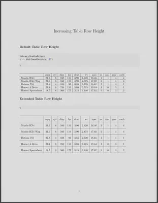
When working with tables, you might want to increase standard row height to add a bit of space. This could make tables easier to read, and it could help a table fit into the overall formatting of a given page.

Adding \renewcommand{\arraystretch}{2} will double the table row height of all subsequent tables. If you want certain tables to have greater row height than others, then you could include this line of code again, replacing 2 with 1 to return row heights to their default.

---
title: "Increasing Table Row Height"
output: pdf_document
---

## Default Table Row Height

```{r}
library(kableExtra)
t <- kbl(head(mtcars, 5))

t
```

## Extended Table Row Height

\renewcommand{\arraystretch}{2}

```{r}
t
```

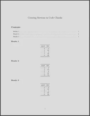
Dynamically Create Sections in Code Chunks

This is a little more involved, but it is perhaps the most powerful trick included in this post. I’ve run into many cases where I’m writing a report, and I need to create identical sections for a given set of data. You probably know how to easily iterate over the data and do the analysis you want, create tables/plots, etc. But then within the iteration, how do you include the results as part of the final document in a coherent manner?

In R Markdown, if you set the chunk option results='asis', the output of your code chunk can be interpreted as LaTeX instead of plain text. This then allows you to call cat() on various objects, such as plots, tables, or even additional markdown or LaTeX, which will then be compiled with the rest of the document.

In other words, you can have a code chunk serve as a section template and create similarly-structured sections dynamically based on your data.

---
title: "Creating Sections in Code Chunks"
output: pdf_document
toc: true
---

```{r echo=FALSE, message=FALSE, results='asis'}
library(tidyverse)
library(kableExtra)
t <- cars %>%
  head(5) %>%
  kbl(booktabs = T) %>%
  kable_styling(latex_options = c("striped", "HOLD_position"))

walk(1:3, function(x) {
  cat("## Header", x, "\n", t)
})
```

Conclusion

I’ve compiled these tips in a single place as much for myself as for others so I have an easy reference document. Being able to take more control over the PDF’s I’m producing has not only made me more effective at my job, but it has also gives me a greater sense of pride in my work-products because I’m able to create the report I want instead of what the defaults dictate. I hope you find similar utility in this post.