Calculating Road Curvature in R

Introduction

A while back I figured out how to access OpenStreetMap data in R, and since then I’ve been a bit obsessed. I’ve created a lot of different graphics (some of which I’ve even had printed and now hang on my walls at home), such as this one below. This is a plot of every road in Wisconsin, and roads are the only thing plotted.

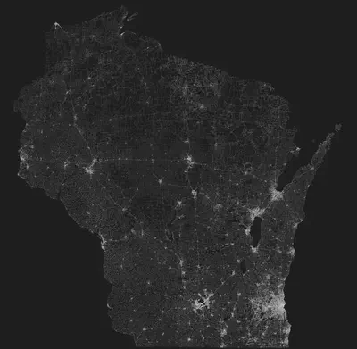
I think images like this are fascinating, and as I was poring over it, I noticed that in certain areas of the state, the pattern of roads gets spidery instead of grid-like (e.g. in the west and north of the state). My knee-jerk hypothesis is that these areas would be topographically different from areas of grid-like roads. In any case, this got me wondering if I could quantify this observation and identify areas of the state with the curviest roads.

So consider yourself warned – this post is about calculating the curvature of roads. Nothing more, nothing less. Buckle up.

The Data

Selecting Road Types

The map above includes all roads in Wisconsin, including service roads (i.e. alleys and parking lots). This is a lot of data, so we should first narrow our focus to make things easier. To understand how we might do this, first we need to know the data source and the basic structure of the data.

I’m sourcing the road data from OpenStreetMap’s Overpass API using the osmdata R package. OpenStreetMap provides A LOT of data, but for our purposes, the important thing to know is that the spatial data for roads is grouped under the highway key, and roads are broken down by the type of road (e.g. motorway, residential, service, etc.). The graphic above includes the following highway types:

• Motorway
• Trunk
• Primary
• Secondary
• Tertiary
• Residential
• Service
• Unclassified

First, let’s consider the type of road we actually want. We want a road that will be curvy in certain areas but strait in others. In other words, we want a road that is responsive to geography, not one that blasts a straight line no matter what. We also want roads that are uniformly present in decent quantities as opposed to roads that are clustered in population centers.

Motorway, Trunk, and Primary roads are major roads such as interstates and highways, which are both sparse and straight. At the opposite end of the spectrum, Service roads are inherently short and curvy, while Unclassified roads can be sparse as well. Residential roads can be sparse as well since they tend to be clustered.

This leaves us with the Secondary and Tertiary roads on which we can focus our attention.

Loading the Data

Now that we’ve identified which road types we want to load, we can build our Overpass query. The code below shows how you can use the osmdata package to write a query.

library(osmdata)

sec_roads <- opq("Wisconsin") %>%
  add_osm_feature(key = "highway", value = "secondary") %>%
  osmdata_sf()

Let’s break this down line by line:

1. First, we have to load osmdata with library(osmdata)
2. Next, the opq() function sets the bounding box for the query, so here we are setting a bounding box around Wisconsin. The query will return all features we specify in subsequent lines within this box.
3. The add_osm_feature() function is the meat of our call here. Overpass queries require key-value pairs to specify data, and here our key is highway and the value is secondary. All roads will be listed under the highway key, and we specify the road type with the value. (For more on the possible OSM feature, see the wiki.)
4. Finally, the osmdata_sf() call will convert the returned data to a type compatible with sf package functions.

Now, this is a pretty simple few lines of code to acquire the data, but my experience is that server errors are quite common when querying OSM for larger chunks of data (e.g. statewide roads), so I have found the best method is to build subsequent queries and save them as they complete. The code below will accomplish this by saving the data to a data folder, but it only makes the query if the particular query data has not been saved already. This way you can run this code subsequently if an error is returned until all data is successfully saved.

road_types <- c("secondary",
                "tertiary")

walk(road_types, function(x) {
  if (!file.exists(paste("data/", x, ".rda", sep = ""))) {
      t <- opq("Wisconsin") %>%
        add_osm_feature(key = "highway", value = x) %>%
        osmdata_sf()
  
    saveRDS(t, file = paste("data/", x, ".rda", sep = ""))
  } else {
    cat(crayon::cyan("All queries complete!"))
  }
})

Once you have the data saved, you won’t have to worry about repeating your Overpass queries. Instead, you just need to read the data into your environment. The code below will accomplis this for you, assuming you followed the steps above.

d_files <- list.files("data")

roads <- map_df(d_files, function(x) {
  cat(crayon::cyan(paste("Starting", x, "\n")))
  t <- readRDS(paste("data/", x, sep = ""))
  cat(crayon::red(paste("Finished", x, "\n")))
  
  if (!is.null(t$osm_lines)) {
    t$osm_lines %>%
      select(geometry)
  } 
})

Note that we are only returning the osm_lines element from the object returned by the query. That is because each query will return available data, but we are only interested in the roads, which are found in the osm_lines element.

Counties

The final piece of we will need is shapefile data for counties so we can aggregate road curvature at the county level. The tigris package in R makes it easy to import the data, but the boundaries along the coastline represent the administrative boundaries, not the actual land boundaries.

For example, the map on the left below shows the administrative boundaries, whereas the one of the right has erased the Great Lakes from those boundaries.

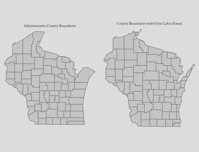
To erase the water from our plot, we can use the rnaturalearth package to import shapefiles for the Great Lakes. A simple st_difference() operation will then cut out the water, leaving a much cleaner map. The code below will handle this for us, and the final counties_trim object will be what we take forward in this analysis. (counties_trim is the same as what was plotted on the right above.)

library(tigris)
library(rnaturalearth)

# Import county shapefile for Wisconsin

counties <- counties(state = "WI")

# Import lakes shapefile

l <- ne_download(type = "lakes", category = "physical", scale = "large")  %>%
  st_as_sf(., crs = set_crs)

# Filter for Great Lakes that border Wisconsin

gl <- l %>% 
  filter(name %in% c("Lake Michigan", "Lake Superior")) %>%
  st_union()

# Match CRS

co <- st_transform(counties, crs = set_crs)

# Erase lakes from counties

counties_trim <- st_difference(co, gl)

Methodology

Now that we have determined what data we will use and loaded said data, we now need to determine what our methodology will be.

Our goal is to quantify the curvature of roads in Wisconsin so we can identify where the curviest roads are located. We have already limited our definition of “road” to mean Secondary and Tertiary roads. Next, we need to define mathematically what we mean by “curvy”.

I will consider here below two methods:

• Method A will be based on the efficiency or directness of the road
• Method B will be based on the angles of the road

Method A: Road Efficiency

Intuitively, we can say that a curvy road is one that does not take a direct path between two points. A road is curvier if it takes a less-direct path than a separate road. By this definition, we could quantify the curvature of a road by dividing the straight-line distance between the start and end points of the road by the full length of the road.

For example, the plot below shows a simple road that travels for one mile in one direction before taking a right-angle turn and continuing for another mile in that direction. This gives the road a total length of two miles.

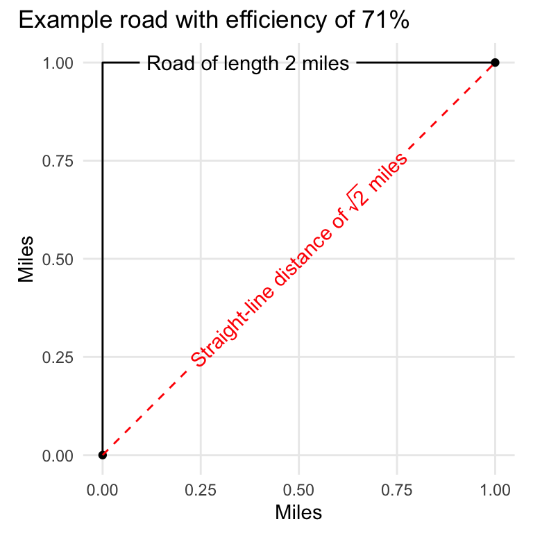
If we connect the start and end points of the road (i.e. the red dotted line), we then have a triangle. If we remember our trigonometry, we know that for a triangle with sides of equal length 1, the hypotenuse will be $ \sqrt{2} $, or 1.414.

The problem here is that an eye check does not tell us that our example road is a curvy road because we do not necessarily consider a road with a single right angle to be a curvy road. This might not be a deal-breaker for this analysis, but let’s still take a look at another method for calculating curvature that better accounts for the actual angles.

Method B: Road Angles

This method will actual measure the angles that are present in the road. To fully understand how this method works, first we need to have a firm grounding in the structure of the road spatial data.

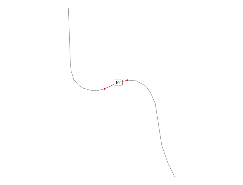
You’ll remember that we extracted the osm_lines element above because it holds the road data, which as you might intuit, are lines. Specifically, they are linestring spatial objects. Linestrings are basically a collection of points that are in a particular order so that a line can be drawn.

Because linestrings are a series of points, we can break a single linestring down to individual lines between two points. If we then consider two consecutive line segments, we can calculate the angle formed by the two lines by connecting the start and end points to form a triangle for which we know the lengths of all sides. We can then then use the law of cosines to calculate the angle.

For instance, the animation below shows an actual road from our data, and the red represents two consecutive segments with the calculated angle labeled at the point of intersection.

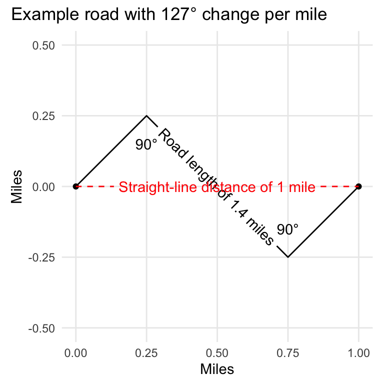
Now that we understand how angles can be calculated along a linestring, let’s look at a basic example to see how we can use this technique to calculate curvature. In the graphic below, we have a road that makes two right angle turns in opposite directions. Since one right angle is 90 degrees, this road exhibits 180 degrees of curves over its entire distance, which is 1.4 miles. If we divide the degrees by the distance, we will have the degree change per mile.

Determination

So, we now have our two methods for quantifying road curvature, but how do they stack up against each other? Looking at our two example roads we’ve considered to this point, we can compare how each method would label them.

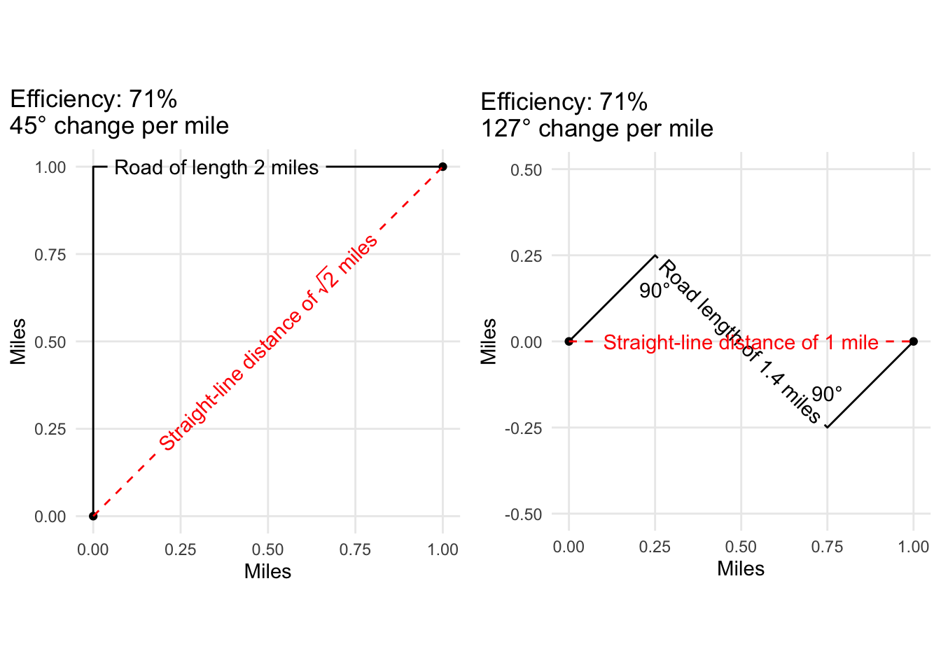
Based on Method A (i.e. the efficiency method), the roads are nearly identical. Method B, though, labels the second road as 180% curvier than the first road! Not only does the second road exhibit more turns, but it also does so in a shorter distance.

By this standard, Method B seems to come out on top. Before we make a final determination, though, let’s do a test run on real data to see what we get. Recall that our data is currently broken in two segments, one for Secondary roads, and one for tertiary.

Implementing the Methods

The code below assumes you loaded the road data into R using the methods described above. If you didn’t follow it exactly, the important goal here is to combine everything in a single dataframe.

# Combine all roads in a single df

r <- bind_rows(roads[[1]], roads[[2]])

Next, we’ll take a sample of this data to test out two methods. I’m choosing to sample 100 rows here – since we’re just testing right now, we don’t want to slow ourselves down by including too much data.

# Create a vector of length 100 for the row indexes

sample_index <- sample(1:nrow(r), size = 100, replace = FALSE)

# Subset the full data with the sample index

sam <- r[sample_index,]

Now, we’re ready to actually implement our methods. I’m not going to get into the nitty gritty of explaining how it works here, but the code below will calculate three things for each road:

• Road length
• Distance between start and end points of road
• Sum of all angles in a road

With these three numbers, we will be able to calculate both the efficiency and the degree change per mile (i.e. Method A and Method B, respectively).

# This code will save a dataframe to `angle` that
# contains necessary measures for Method A and
# Method B.

angle <- map_df(1:nrow(sam), function(x) {
  # Print to console, this really helps with debugging
    cat(crayon::cyan("Starting Road", x, "  "))
  
  # Isolate geometry of this road
    t_ <- sam[x,"geometry"]
    
    # Limit to LINESTRINGS -- this is more important
    # for later in the analysis when we are breaking
    # things up by counties, which could create edge 
    # cases of other types of geometries, which won't 
    # work here.
    
    if (st_geometry_type(t_) == "LINESTRING") {
      cat(crayon::white("LINESTRING\n"))
      
      # Extract points from the LINESTRING
      t_points <- st_cast(t_, "POINT")
      
      ############
      # Method A #
      ############
      
      # Calculations for Method A are pretty simple
      # Distance between start and end points
      dist <- st_distance(t_points[1,], t_points[nrow(t_points),])
      
      # Full length of road
      l_length <- st_length(t_)
      
      # Count of points in LINESTRING
      # This is informative but not entirely necessary for 
      # our calculations.
      point_count <- nrow(t_points)
      
      ############
      # Method B #
      ############
      
      # This calculates the angles. Two consecutive 
      # segments of the actual road form two sides of
      # a triangle, and the third side is created by 
      # connecting the start and end points. From there,
      # knowing the length of all triangle sides, we can
      # calculate the angles.
      
      if (nrow(t_points) > 2) {
        angles <- map_df(3:nrow(t_points), function(p) {
          
          # Calculate triangle side lengths
          seg <- t_points[c((p - 2):p),]
          ab <- st_distance(seg[1,], seg[2,])
          bc <- st_distance(seg[2,], seg[3,])
          ac <- st_distance(seg[1,], seg [3,])
          
          # Law of cosines to calculate angle
          angle <- acos(
            (ac^2 - ab^2 - bc^2) / (-2 * ab * bc)
          )
          
          tibble(
            # Angle was in radians, conver to degrees
            angle = 180 - (as.numeric(angle) * 180 / pi),
            end_index = p,
          )
          
        })
        
        # Sum of all angles present in the LINESTRING
        tot_angle <- sum(angles$angle, na.rm = TRUE)
        
        # This is our export, which includes all the
        # measures necessary for both Method A and 
        # Method B.
        df <- tibble(dist = dist,
                     l_length = l_length,
                     point_count = point_count,
                     tot_angle = tot_angle,
                     ind = x)
      } else {
        #  Can't calculate angles with only two points
        cat(crayon::red("Two or fewer points.\n"))
      }
    } else {
      # This evaluates if the geometry isn't a LINESTRING
      cat(crayon::red("Not a LINESTRING.\n"))
    } 
})

The final step for us is to calculate our actual method measures, which is accomplished with the code below.

af <- angle %>%
  mutate(efficiency = as.numeric(dist / l_length),
         angle_rate = tot_angle / dist) 

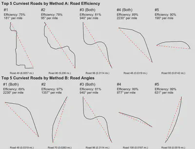
And there we have it! Now we can compare the curviest roads as defined by each measure. The figure below shows the top five curviest roads by Method A on top and Method B on bottom.

Final Determination

Method A seems to be effectively identifying curvy roads, whereas Method B obviously shows a bias for shorter lengths of road. Method B would be the method of choice for identifying particular segments of road that exhibit the greatest curvature, and it would theoretically work for our purposes here in the aggregate – i.e. calculating the road angle change for an entire county would mitigate this bias.

There is, however, a very important consideration that I have yet to mention, and that is computational cost. As it turns out, Method B takes 27 times as long as Method A! If we think about it, this isn’t all that surprising since Method B performs calculations for each point in a linestring, whereas Method A is really only concerned with the start and end points of a line, regardless of length.

To put this in perspective, it took my machine (with 32 GB RAM) over 30 seconds to process 100 observations using Method B. Considering the full data set contains over 47,000 observations, we can estimate that it would take 235 minutes, or about 4 hours, and that’s probably an optimistic estimate since there are undoubtedly roads with many more points than in our sample (and it’s the point count that determines the processing time).

Because Method A is adequately identifying curvy roads, and because it much more efficient, we will select Method A for our actual analysis.

Analysis

We’ve now reached a point where most of the hard work is done – we’ve identified and sourced our data, we’ve evaluated and selected our methodology, and we have our geographic grouping data in our counties_trim object.

As we saw when we tested our methodologies, the actual analysis will be accomplished by iterating over every row in our dataframe of roads, which you’ll recall is stored in our r object.

Since we’re looking at the county level, our iteration will be nested inside an iteration over the counties. In other words, for each county, we will iterate over all roads in that county. The code below accomplishes this for us.

all_wi <- map_df(1:nrow(counties), function(c) {
  one_c <- co[c,] 
  county <- one_c$NAME
  
  p_county <- st_intersection(r, one_c)
  
  temp_ <- map_df(1:nrow(p_county), function(x) {
    cat(crayon::cyan("Starting County", c, "Road", x, "  "))
    t_ <- p_county[x,"geometry"]
    
    # Extract LINESTRINGS from GEOMETRYCOLLECTION
    if (st_geometry_type(t_) == "GEOMETRYCOLLECTION") {
      t_ <- st_collection_extract(t_,type = c("LINESTRING"))
    }
    
    if (st_geometry_type(t_) == "MULTILINESTRING") {
      t_ <- st_cast(t_, "LINESTRING")
    }
    
    # Handle LINESTRINGS
    if (st_geometry_type(t_[1,]) == "LINESTRING") {
      cat(crayon::white(paste0(st_geometry_type(t_), "\n")))
      
      map_df(1:nrow(t_), function(ml) {
        sub_l <- t_[ml,]
        t_points <- st_cast(sub_l, "POINT")
        
        dist <- st_distance(t_points[1,], t_points[nrow(t_points),])
        l_length <- st_length(sub_l)
        point_count <- nrow(t_points)
        
        df <- tibble(dist = dist,
                     l_length = l_length,
                     point_count = point_count,
                     county = county)
      })
      
    } else {
      cat(crayon::red(paste0("OTHER GEOMETRY: ", st_geometry_type(t_), "\n")))
    }
  })
  
  return(temp_)
})

There are a couple things I wont to point out about this code:

• Not every element is a LINESTRING, so the callback function needs to be able to handle those cases. Essentially, it attempts to extract any LINESTRING elements while excluding other elements.
• In the case of MULTILINESTRING elements, we break those up into individual LINESTRING elements. This is important because a single road could be broken up into disconnected segments for a variety of reasons (e.g. intersections are categorized as different road types, the road traverses county boundaries, etc), and this could result in a road having an efficiency greater than 100%. Wormholes notwithstanding, this is obviously impossible and undermines our analysis.
• The output is a dataframe that includes a row for each individual LINESTRING element with columns for its county, its length, its distance between start and end points, and its point count.

From here, it’s a simple matter of summarizing our all_wi dataframe to calculate the county-level road efficiency. We do this by dividing the sum of all road lengths in the county by the sum of distance between start and end points of all roads.

aw_summed <- all_wi %>%
  group_by("NAME" = county) %>%
  summarise(total_eff = sum(dist, na.rm = TRUE) / sum(l_length, na.rm = TRUE)) 

Results

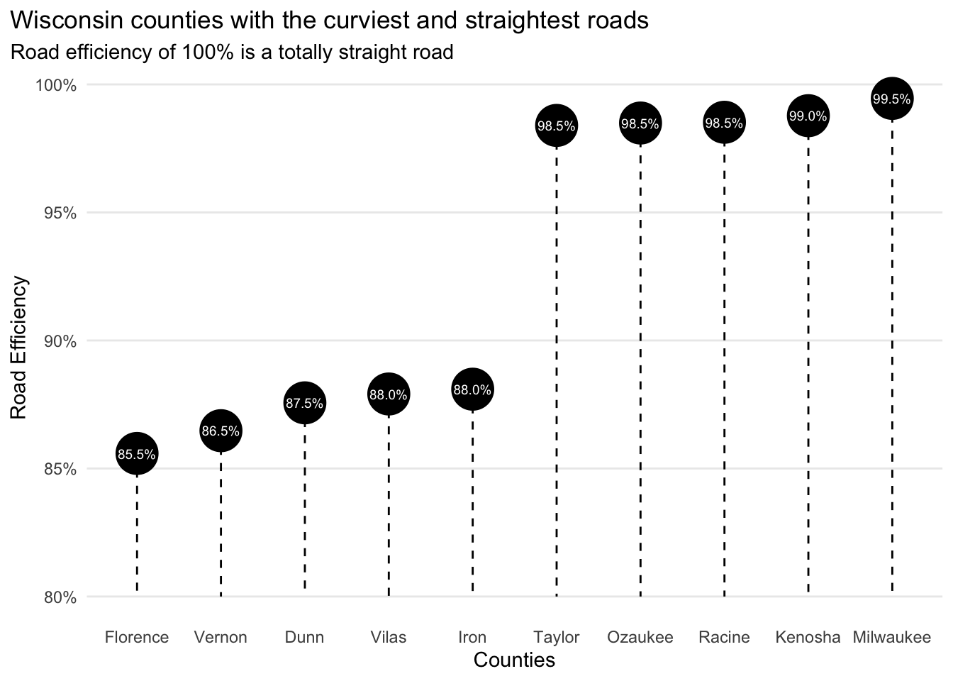
So where are the curviest roads? As the plot below portrays, Florence County has the curviest roads, and Milwaukee County has the straightest roads. (The plot includes the 5 curviest and 5 straightest roads.)

Seeing Milwaukee has the straightest roads is a little validating since Milwaukee is a heavily developed area with many grid-like road layouts, but what does the picture look like statewide?

The figure below whos the counties with the curviest roads in dark green and the straightest roads in light green.

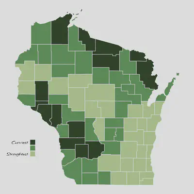
If you know a bit about Wisconsin’s geography, you know that the western edge of the state is the Driftless Area, and the north is the Northwoods. Both of these areas are geographically dynamic, so it makes sense that they are home to the curviest roads in the state. This also lines up with the roads plot that inspired this whole analysis.

So, I’m declaring this a success!