Getting Creative with Spatial Buffers
TL;DR
Bisect a spatial polygon with a spatial line using sf::st_buffer() with singleSide=TRUE. For example, consider a road that runs east-west and bisects a city. Buffer on one side of that road to create a polygon that includes all portions of the city north or south of the road.
If you’re familiar with sf and st_buffer(), skip down to the What I learned section.
Introduction
Have you ever used a function in R for such a long time that you’re sure you know its capabilities, and then you find out you missed a key bit of functionality? This happened to me recently with the sf::st_buffer() function–I didn’t realize you could limit a buffer to a single side!
The purpose of this post is threefold:
- Explain the basic usage of the
sf::st_buffer()function - Introduce the functionality that I missed (limiting a buffer to one side)
- Show usage of that functionality and why it’s handy
This post is going to assume you have basic familiarity with the sf package. This is a fantastic package that makes it pretty simple to work with spatial data in your tidy workflows–learn more about the package on its website here.
Data prep
I’m going to load the data we’ll be using in this post now so we can use it in examples throughout. The examples are going to be based on polling locations in the city of Milwaukee, Wisconsin, and we’re also going to make use of road locations. The next few code chunks will get us set up for the rest of the post.
Load packages
# Code in this post will be using these packages,
# let's load them now
library(tidyverse)
library(sf)
library(glue)
library(tigris)
Get polling locations
# download polling places for Milwaukee from data.milwaukee.gov
url <- "https://data.milwaukee.gov/dataset/3c87875e-cf75-4736-a01b-fbf3e889d0b0/resource/a039829e-b578-4ce1-92cc-5ded8bc38c71/download/pollingplace.zip"

destdir <- tempdir()
utils::download.file(file.path(url), zip_file <- tempfile())
utils::unzip(zip_file, exdir = destdir)

# list files in `destdir` to see file name
# list.files()

# read in file
polls <- st_read(glue("{destdir}/pollingplace.shp"))
## Reading layer `pollingplace' from data source
##   `/private/var/folders/91/qhfp3fn13f9411wvjnhhszxc0000gn/T/RtmpoYY0RI/pollingplace.shp'
##   using driver `ESRI Shapefile'
## Simple feature collection with 180 features and 7 fields
## Geometry type: POINT
## Dimension:     XY
## Bounding box:  xmin: 2517465 ymin: 348252.8 xmax: 2567484 ymax: 440084.2
## Projected CRS: NAD27 / Wisconsin South
Milwaukee city limits
# Milwaukee city limits
wi_places <- tigris::places(state = "wisconsin")
mke <- wi_places |>
  filter(NAME == "Milwaukee") |>
  # make same CRS as `polls`
  st_transform(crs = st_crs(polls))
Milwaukee roads
# Download roads in Milwaukee using the `tigris` package
mke_roads <- roads("wisconsin", county = "Milwaukee")

# make same CRS as `polls
mke_roads <- st_transform(mke_roads, crs = st_crs(polls))

# Filter for interstates
mke_int <- mke_roads |>
  filter(str_detect(FULLNAME, "^I- "))
Review
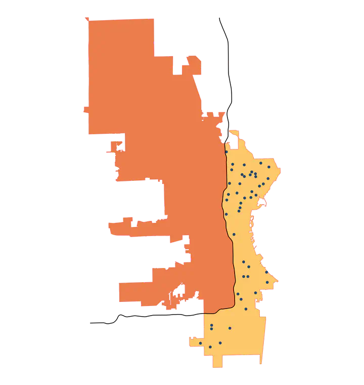
# Plot the data to get a visual of our data
mke |>
  ggplot() +
  geom_sf() +
  geom_sf(data = mke_int) +
  geom_sf(data = polls, size = .75, color = "red") +
  theme_void()

Usage
The st_buffer() function creates a buffer around a spatial object. You provide a spatial object, specify the distance of the buffer, and st_buffer() adds your specified space between the bounds of the original object to create counts of a new spatial object. This is easy to understand with examples.
Points
Let’s take a random point from our polls data to show what buffering around a point does.
# select a single point
one_point <- polls[1,]

# buffer around the point
buff_point <- st_buffer(one_point, dist = 10)

# plot both point and its buffer
one_point |>
  ggplot() +

  # plot the buffer layer first so it doesn't cover point
  geom_sf(data = buff_point, fill = "yellow", color = "yellow") +

  geom_sf(color = "blue")
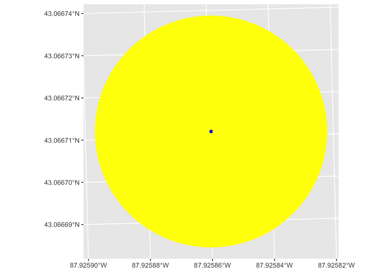
We see that this creates a circle centered on our point with a radius of the dist we set in st_buffer(), in this case 10.
Lines
Now let’s do the same thing with lines using our mke_int data.
# select a single line
# selecting the 2nd row because it's a better example than the first
one_line <- mke_int[2,]

# buffer around the line
buff_line <- st_buffer(one_line, dist = 10)

# plot both line and its buffer
one_line |>
  ggplot() +
  geom_sf(data = buff_line, fill = "yellow", color = "yellow") +
  geom_sf(color = "blue", linewidth = 1)
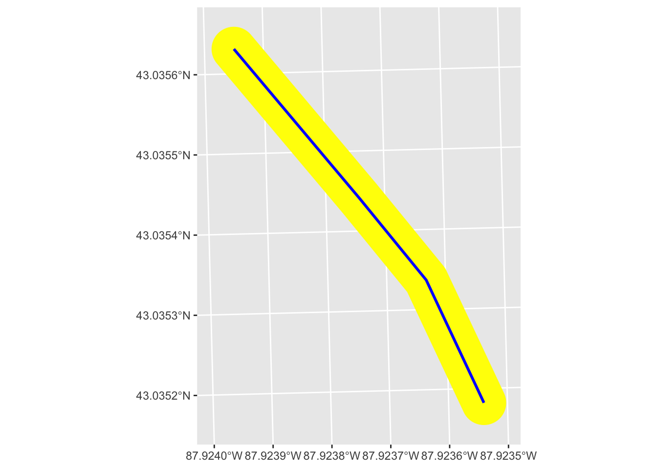
This buffer is doing the same thing as we saw with the point, except it’s doing it along the length of the line. The result is that our new buffer polygon extends the dist we specified perpendicular to the original line. The width of the new polygon then is twice what we set for dist.
Polygons
Finally, let’s do the same with the mke polygon.
# `mke` is already just one polygon, so don't need filter
# just need to create a buffer
# since the scale of this polygon is bigger, we need to set
# the `dist` argument bigger
buff_poly <- st_buffer(mke, dist = 1000)
# plot both polygon and its buffer
mke |>
ggplot() +
geom_sf(data = buff_poly, fill = "yellow") +
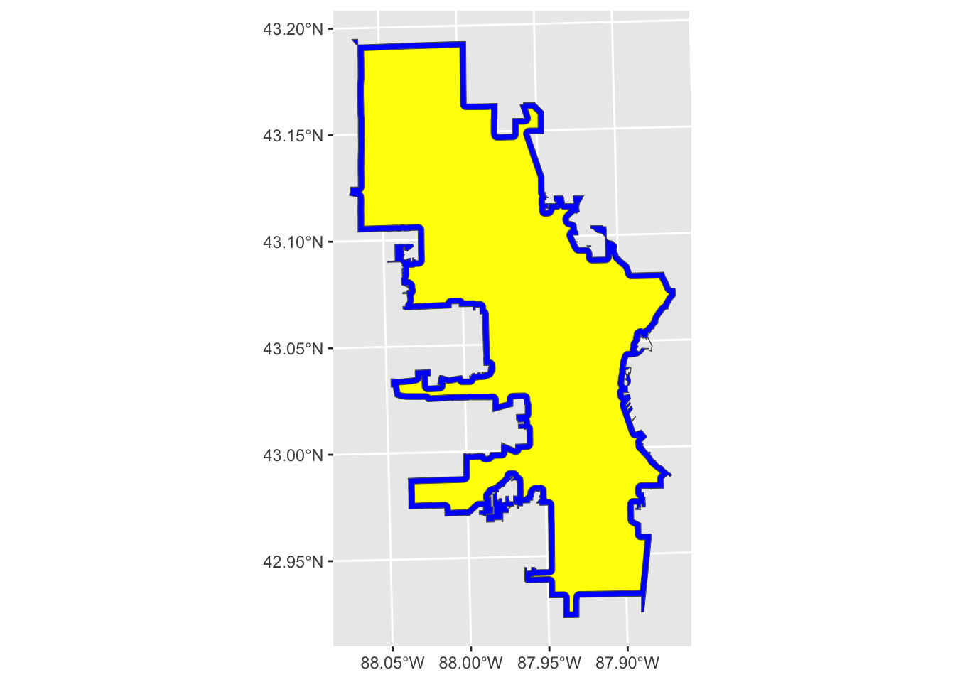
geom_sf(fill = "blue")
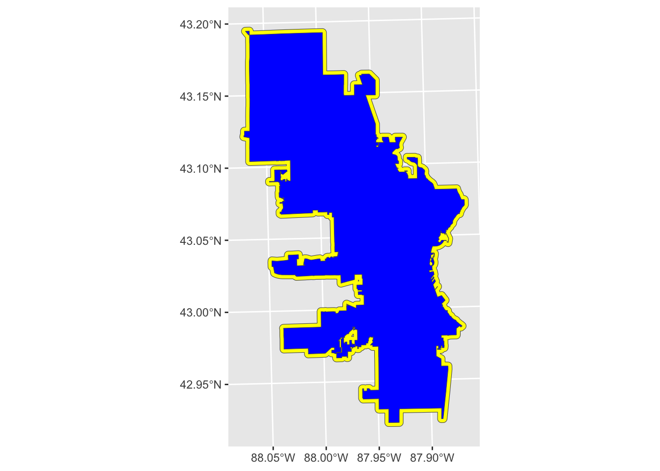
This buffer extends the designated dist from the boundary line and in that way is similar to the line buffer. One difference with polygon buffers is that we can also do negative distances, which will buffer to the inside, resulting in a smaller polygon than the original.
# Let's use a negative buffer this time
neg_buff_poly <- st_buffer(mke, dist = -1000)

# plot both polygon and its buffer
# need to reverse order of layers so bigger one is on top
mke |>
  ggplot() +
  geom_sf(fill = "blue") +
  geom_sf(data = neg_buff_poly, fill = "yellow")
Now our plot looks like the border is blue and the polygon is yellow, but the blue actually shows the original polygon (i.e., Milwaukee city limits), and the yellow shows a negative buffer, or a buffer inside the polygon.
Units
So far, we have been setting the dist argument of st_buffer() as a number without mentioning units. You are not required to designate units because sf will assume the units based on the Coordinate Reference System (CRS).
You’ll notice above when I loaded the data that I used st_transform() to set the CRS of mke and mke_int to the same as poll. This way, we ensure that all spatial objects are using the same CRS. You can also use st_crs(polls) to review the details of the CRS, but a quick way to find out the units is with st_distance(), which will return the distance of a line with units.
# return the distance of `one_line` with units
st_distance(one_line)
## Units: [US_survey_foot]
##      [,1]
## [1,]    0
We see that the unit being used is the US survey foot.
What I learned
So far, we’ve reviewed the basics of the st_buffer() function. I’ve gone several years now thinking this function was limited to what I described above, and it has served me well. Recently, though, I took the time to read more of the documentation, and I had a minor Eureka! moment.
In the documentation (see ?sf::st_buffer), I realized there was an argument I had been overlooking: singleSide. The documentation tells us that if this argument is set to TRUE, the buffer for a line will be limited to one side of the line. Negative values will buffer on one side, positive on the other.
For example, let’s try it with our one_line from above.
# Single-sided buffer of the same line used above
buff_sided <- st_buffer(one_line, dist = 10, singleSide = TRUE)

one_line |>
  ggplot() +
  geom_sf(data = buff_sided, fill = "yellow", color = "yellow") +
  geom_sf(color = "blue", linewidth = 1)
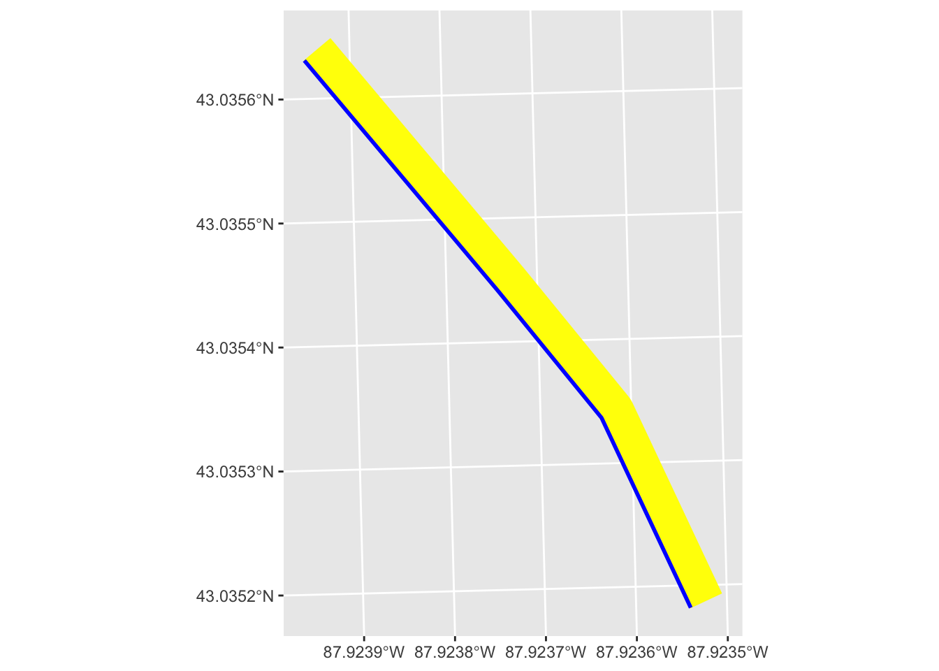
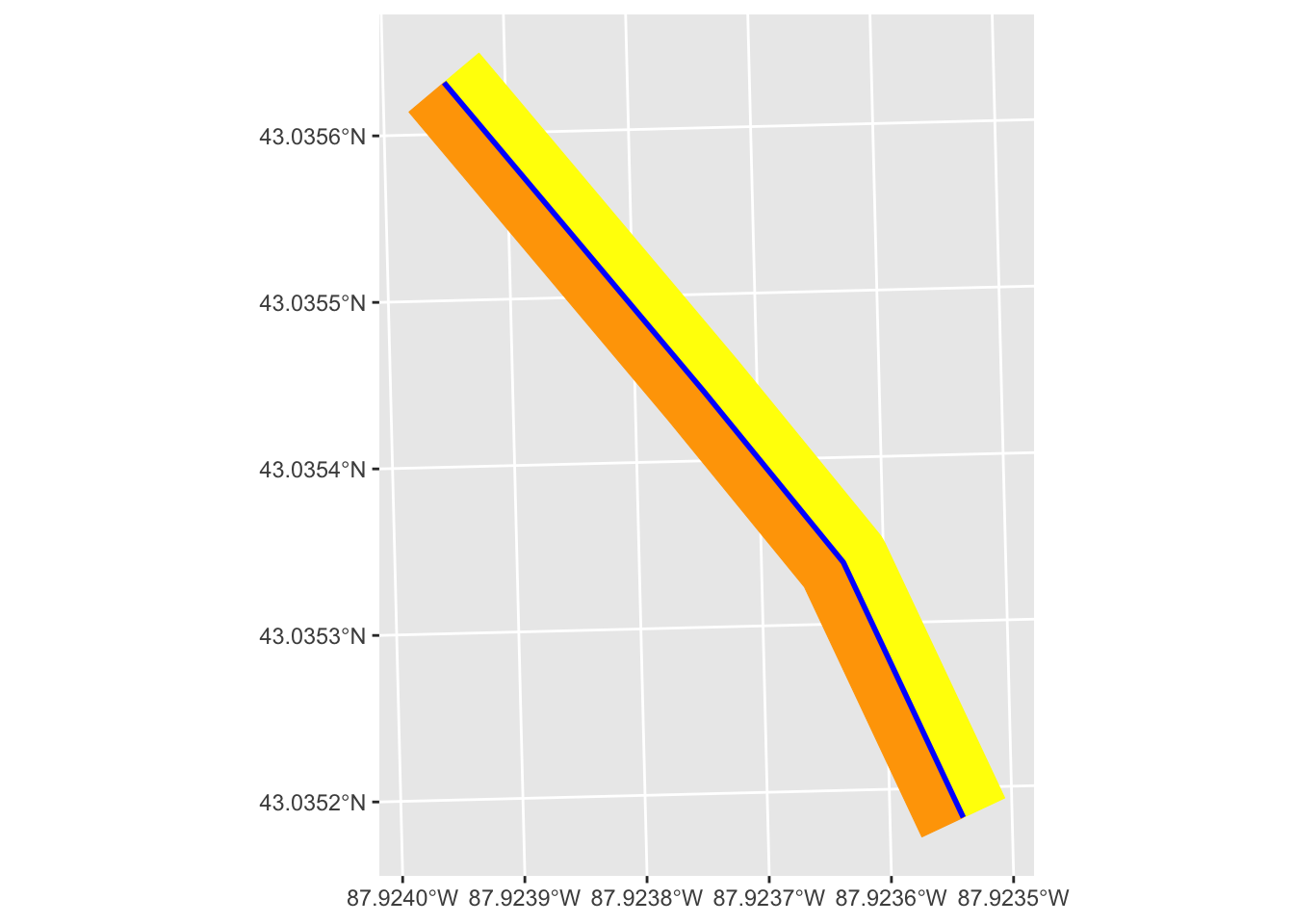
We see that the buffer (in yellow) is only applied to one side of the line. We can also set a buffer on the other side.
# Single-sided buffer of the same line used above
buff_sided_neg <- st_buffer(one_line, dist = -10, singleSide = TRUE)

one_line |>
  ggplot() +
  geom_sf(data = buff_sided, fill = "yellow", color = "yellow") +
  geom_sf(data = buff_sided_neg, fill = "orange", color = "orange") +
  geom_sf(color = "blue", linewidth = 1)
Example use cases
You might be thinking, so what?–what’s the big deal about being able to do a single-side buffer?
One use case that I have personally encountered on numerous occasions is as follows:
- I’m working with spatial points within a spatial polygon (e.g., polling locations in a city)
- I want to isolate points on one side of a spatial line that bisects the polygon (e.g., polling locations that are east of an interstate in a city)
- It seems like I should be able to combine the line (an interstate) with the polygon to essentially cut it in half
Before I fully read the documentation for st_buffer(), all my attempts at this had failed. It is, of course, much easier than I was making it using this simple feature of st_buffer().
Let’s look at our data again:
# Plot the data to get a visual of our data
mke |>
  ggplot() +
  geom_sf() +
  geom_sf(data = mke_int) +
  geom_sf(data = polls, size = .75, color = "red") +
  theme_void()
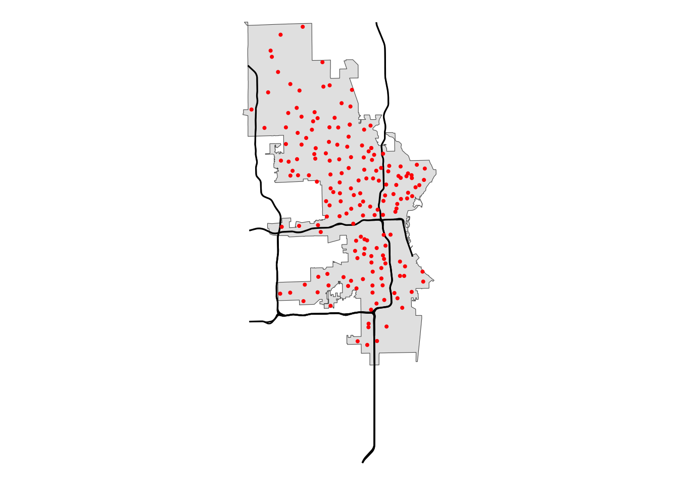
Say we want to look at polling locations that are east or south of Interstate 43. First, let’s limit our interstate data.
# filter for I43
i43 <- mke_int |>
filter(FULLNAME == "I- 43") |>
# to simplify, let's take the main line
mutate(ind = row_number()) |>
filter(ind == 1)
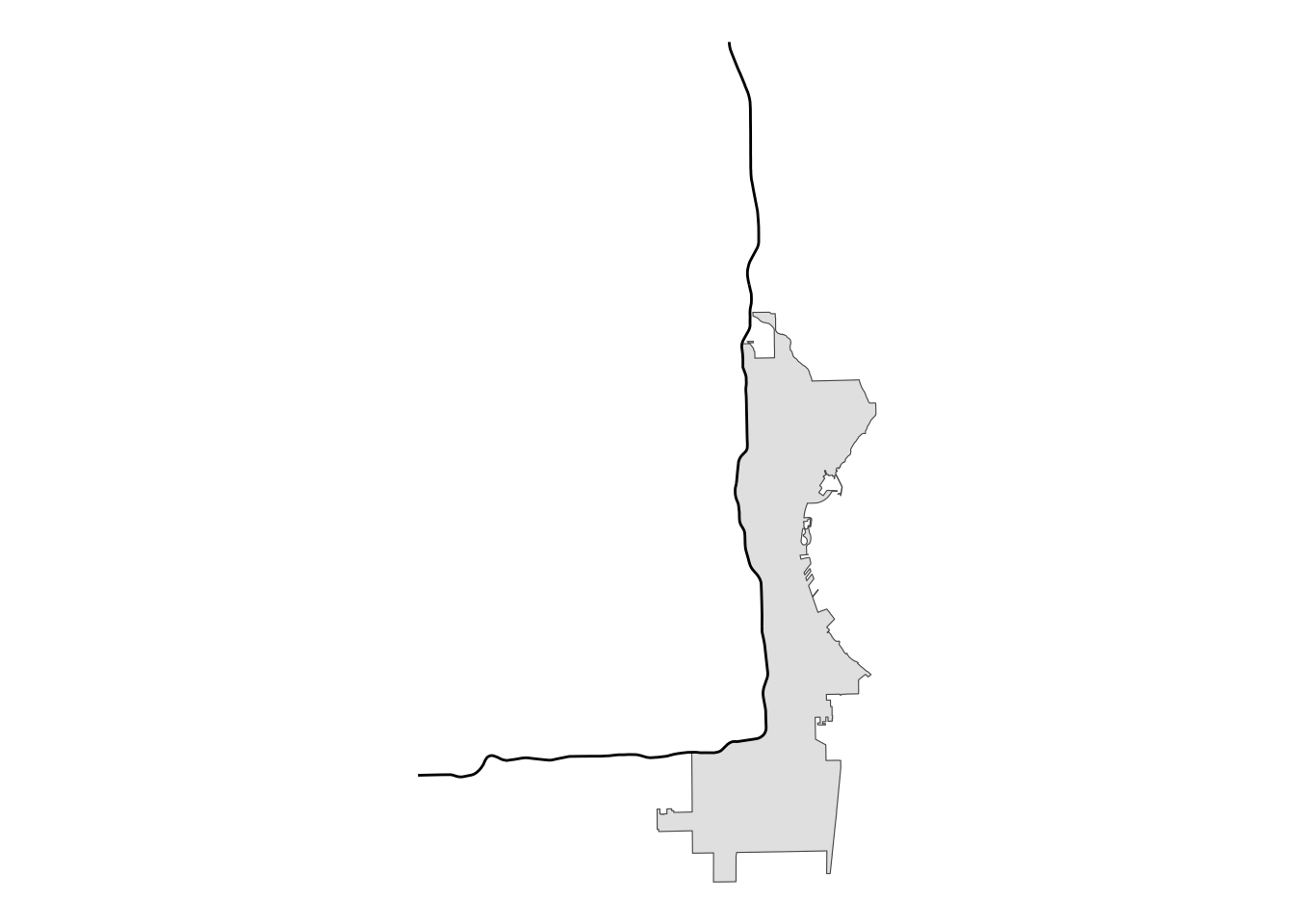
i43 |>
ggplot() +
geom_sf(data = mke) +
geom_sf() +
theme_void()
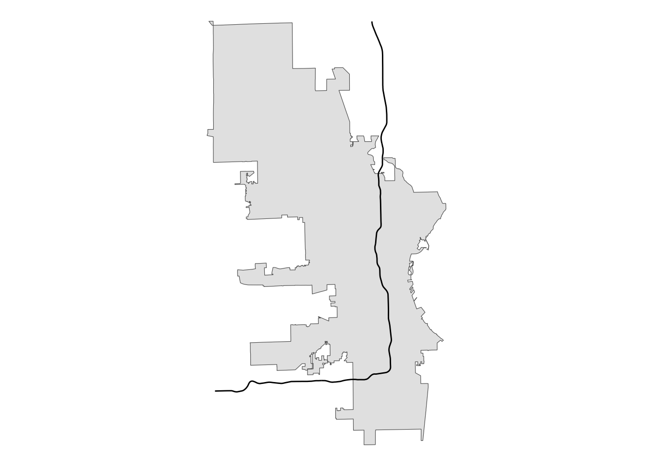
My original thinking was that sf must have a way to take a line like we have here that totally bisects a polygon and create one or two new polygons based on those points of intersection.
We can create a buffer from the interstate that extends beyond the city limits, but using a two-sided buffer won’t work because that will create a new polygon whose edge is not the original line.
# create buffer around interstate
two_sided <- st_buffer(i43, 20000)

# plot for review
two_sided |>
  ggplot() +
  geom_sf(data = mke) +
  # using alpha so we can see underlying boundaries
  geom_sf(color = "yellow", fill = alpha("yellow", .5)) +
  geom_sf(data = i43) +
  theme_void()
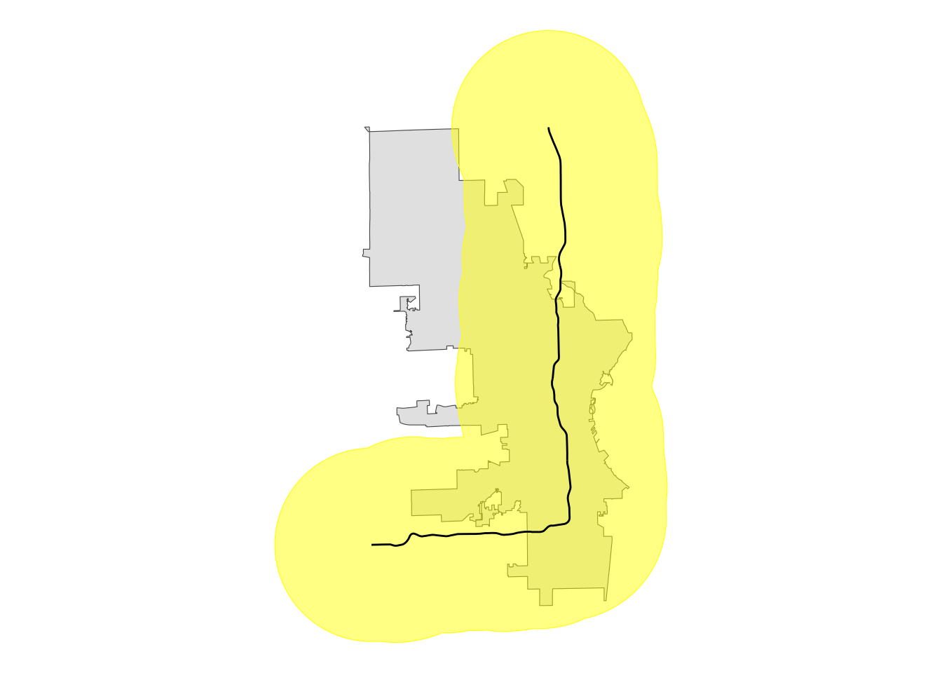
This buffer covers all the area of city limits east and south of the interstate, but it extends well north and west, too. This won’t work for our purposes because an intersection (st_intersection()) will include all that area.
# use st_intersection to clip city limits
city_int <- st_intersection(mke, two_sided)

# plot for review
city_int |>
  ggplot() +
  geom_sf() +
  # using alpha so we can see underlying boundaries
  geom_sf(data = i43) +
  theme_void()
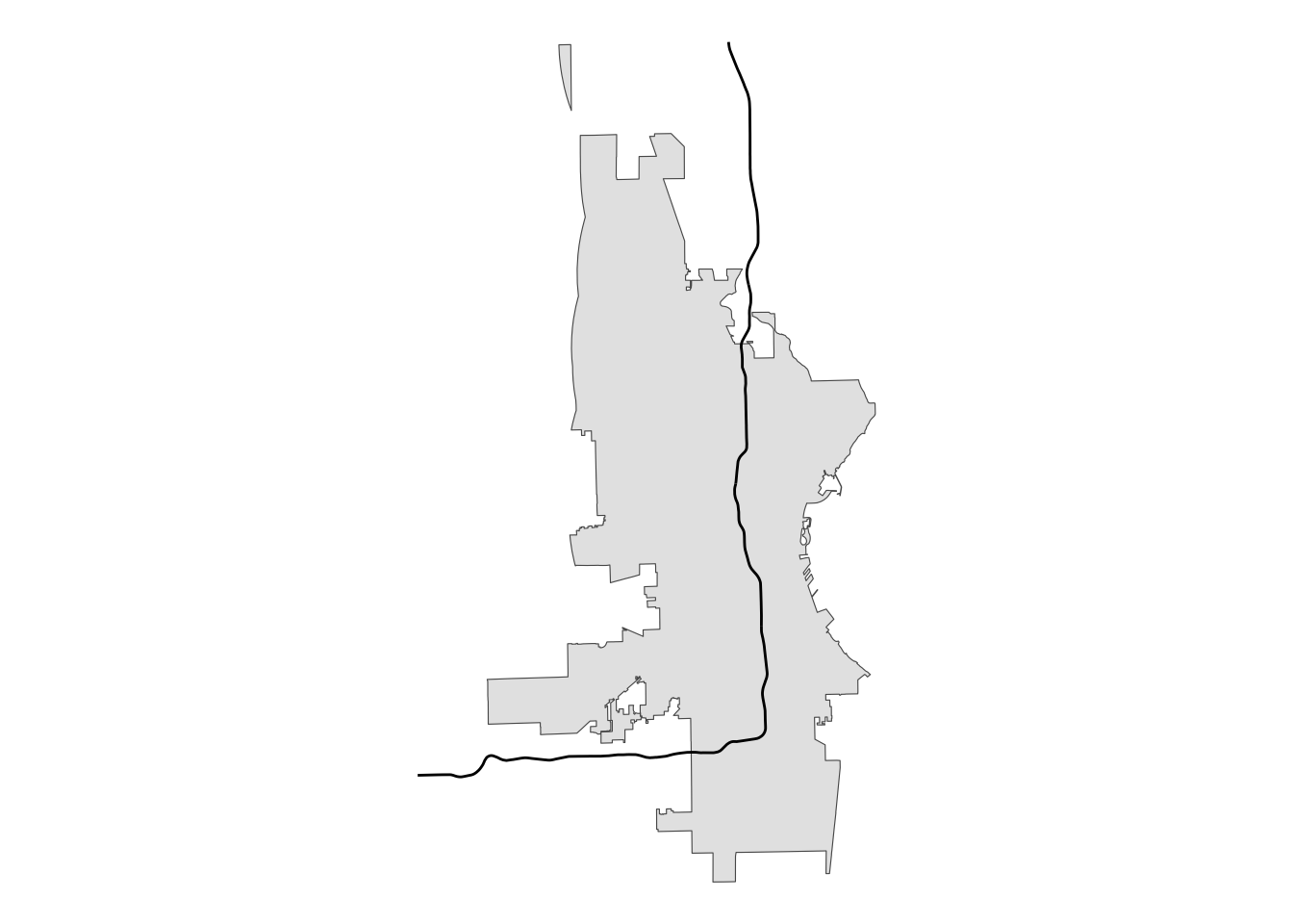
This is not what we want. So, here is where the singleSide option comes in handy.
# single-sided buffer
single_sided <- st_buffer(i43, -20000, singleSide = TRUE)

# plot for review
single_sided |>
  ggplot() +
  geom_sf(data = mke) +
  # using alpha so we can see underlying boundaries
  geom_sf(color = "yellow", fill = alpha("yellow", .5)) +
  geom_sf(data = i43) +
  theme_void()
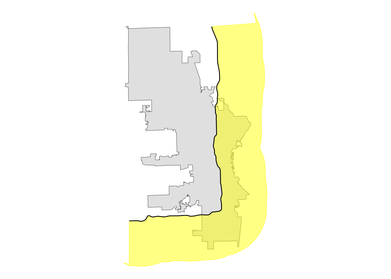
That gives us what we want! Now we can use that buffer polygon to intersect with the city polygon to create a new polygon that represents the portion of the city east and south of Interstate 43.
# create intersection with city limits
se_mke <- st_intersection(mke, single_sided)

# plot for review
se_mke |>
  ggplot() +
  geom_sf() +
  geom_sf(data = i43) +
  theme_void()
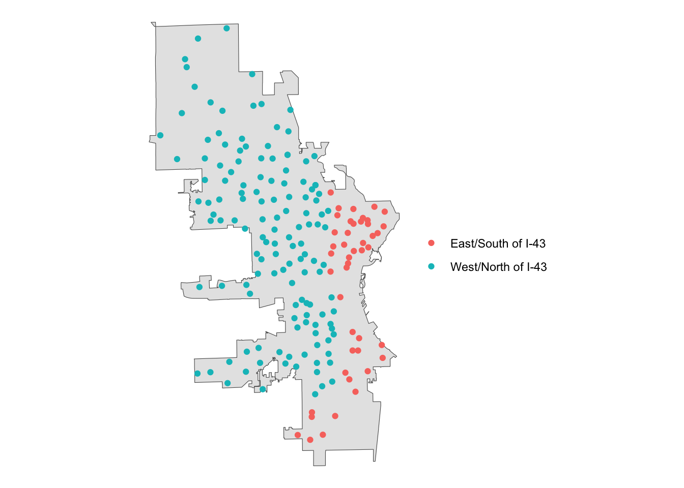
Perfect! Now that we have our section of the city defined, we can join with the polls data to identify which polling locations are in this area.
# join the polls data with se_mke to ID those polls
se_polls <- st_join(polls, se_mke)

# plot for review
se_polls |>
  # create an indicator variable
  mutate(our_polls = ifelse(!is.na(ind), "East/South of I-43", "West/North of I-43")) |>
  ggplot() +
  geom_sf(data = mke) +
  geom_sf(aes(color = our_polls)) +
  theme_void() +
  labs(color = "")
Conclusion
Personally, I was exhilarated when I figured out how to do this kind of spatial operation. It had been limiting me in small but annoying ways for a while, and finding a solution made me feel…capable.
I hope you find this post informative and useful, but more than that, I hope if makes you feel a little bit more capable.
Spencer Schien
Senior Manager of Data & Analytics
This is my bio. There are many like it, but this one is mine.